3
$\begingroup$

I have the solution to this problem but I don't really understand it.

Let $f_X(x) = \dfrac {1}{10}, \ x = 0, 1, 2, ... 9$ and $h(Y|x) = \dfrac {1}{10-x}, y = x, x+1, x+2, ..., 9$.

a) Find $f(x, y)$.

b) Find $f_Y(y)$


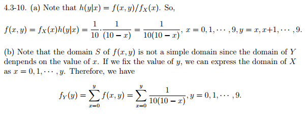
This is the solution my professor posted:

I am having trouble understanding part b). As I recall, $\displaystyle f_Y(y) = \sum_{x \in S_x}f(x, y)$. I see that $S_Y$ is not fixed, but $S_X$ is. So why did my professor write $f_Y(y) = \displaystyle \sum_{x=0}^y \dfrac {1}{10(10-x)}$ instead of $f_Y(y) = \displaystyle \sum_{x=0}^{9} \dfrac {1}{10(10-x)}?$ The first one seems to imply that the domain of $x$ is not fixed.


EDIT: As I was writing this question, I think I may have figured it out, but I would still like confirmation please that I am correct:

Take $y = 3$ as an example.

$\displaystyle f_Y(y) = \sum_{x \in S_x}f(x, y) = f(0, 3) + f(1, 3) + f(2, 3) + f(3, 3) + f(4, 3) + f(5, 3) + f(6, 3) + f(7, 3) + f(8, 3) + f(9, 3) = \sum_{x=1}^3 \dfrac {1}{10(10-x)} + 0 + 0 + 0 + 0 + 0+0$

$\endgroup$

1 Answer 1

4
$\begingroup$

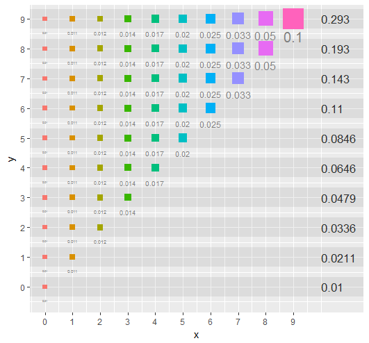
One of the best ways to reason with joint distributions is to draw a picture. Figure

Because this situation involves a discrete distribution, the picture plots the individual probabilities, $f_{X,Y}(x,y)$. It represents the probability of each possible $(x,y)$ with a square symbol whose area is proportional to the probability. All nonzero probabilities are posted beneath each symbol, as computed in part $(a)$ of the solution.

This picture was constructed by taking each possible value $x=0, 1, \ldots, 9$ in turn and plotting the values of $y$ where the probabilities are nonzero. For instance, when $x=4$ the possible values of $y$ are $y=4,5,\ldots, 9$: these appear as a vertical line of dots ascending from $(4,4)$ to $(4,9)$.

The marginal probabilities for $Y$, $f_Y(y)$, are found by summing across all $x$ for each possible value $y$, as computed in part $(b)$ of the solution. Those sets of possibilities are outlined in darker strips. The sums of the probabilities within those strips are posted at the right.

Finding the marginal distribution $f_Y$ is thereby exhibited as a geometrical process of cutting the picture into horizontal strips and collecting the probabilities within each strip.


This is a common theme in many bivariate probability problems: probabilities are specified or constructed by fixing one variable and changing the other (here, fixing $X$ and changing $Y$) but the question requires fixing a different variable (here, fixing $Y$ and changing $X$). A two-dimensional plot like this helps coordinate those operations correctly.

$\endgroup$
0

Your Answer

By clicking “Post Your Answer”, you agree to our terms of service and acknowledge you have read our privacy policy.

Not the answer you're looking for? Browse other questions tagged or ask your own question.