Predicting time to event, conditional on time-varying covariates and survival to time t

Question

In R, I am trying to use a Weibull model to generate predictions of the time to an event, conditional on a set of time-varying covariates and survival to time t. This is partly a coding question, but it's also a methods question, and I can't share my data to make a reproducible example, so I thought I would post it here instead of Stack Overflow.

Using survreg, I can get predicted responses from a fitted model for any given vector of covariate values. The predictions produced by predict(fitted.weibull.model, type = 'response'), however, appear to be unconditional, i.e., not tied to the survival times reported in the associated rows. That's true whether I'm computing in-sample estimates or applying the model to new data.

I had assumed, apparently incorrectly, that for parametric models predict.survreg would also account for the model-estimated duration dependency. For example, if the model showed a secular increase in the likelihood of event occurrence with the passage of time, then a series of predicted responses generated from that model for a given individual would shrink as her survival time increased, assuming that other time-varying covariates remained constant. But that's not what I see in my results.

Is this even a thing? If so, is there a canned way to do this in R, or is it one of those things where you've got to roll your own function to combine the unconditional predictions with the duration-dependency component to get forecasts conditional on observed survival times? If it's a roll-your-own situation, can anyone point me toward a worked example, ideally but not necessarily in R? My searches have come up empty.

Answer 1

Although I don't have a solution that involves survreg, the spduration package has split-population duration regression models that allow you to predict conditional on t and a set of time-varying covariates. Here is an example using code from ?spdur, which estimates a model of the time to a successful coup d'etat, using polity 2 regime scores as the only predictor in both the duration and risk equations:

library(spduration)
data(coups)

# Add duration data related variables
dur.coups <- add_duration(coups, "succ.coup", unitID="gwcode", tID="year",
                      freq="year")

# Focus on one case in the original data, we will replicate this row 10 times and 
# pretend t changes over that time
df <- dur.coups[2, c("gwcode", "year", "polity2", "failure", "ongoing", "end.spell", "atrisk", "censor", "duration", "t.0")]
df <- df[rep(1, 10), ]
df$duration <- 1:10
df$t.0 <- 0:9

# Example model with Polity2 score as only predictor in both equations

# Estimate model
model.coups <- spdur(duration ~ polity2, atrisk ~ polity2, data = dur.coups)

condhaz <- predict(model.coups, newdata = df)
plot(1:10, condhaz, type = "l", xlab = "t", ylim = c(0, .05))
title(main = "Polity2 in duration and risk equation")

# try same data/model with other values for polity2
df_i <- df
cols <- colorRampPalette(c("red", "blue"))(n=21)
for (p2 in -10:10) {
  df_i$polity2 <- p2
  condhaz_i <- predict(model.coups, newdata = df_i)
  lines(1:10, condhaz_i, col = cols[p2+11])
}

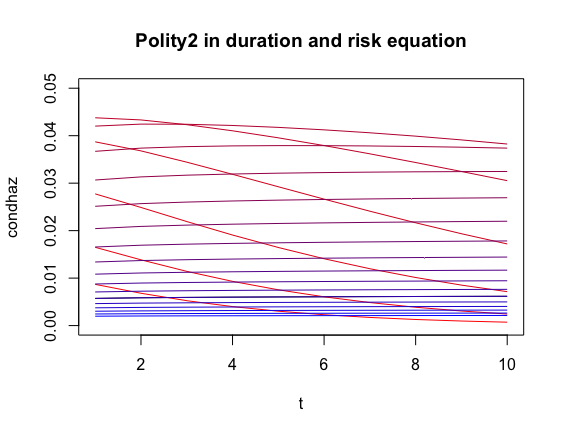
The resulting plot shows how the conditional hazard for countries with different Polity2 values (that themselves are constant over time) evolve over assumed survival time t:

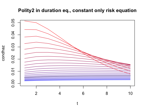
The plot is more complicated than one might expect with a Weibull hazard shape because the predictor Polity2 is in both the duration and risk equations. There is no plain Weibull regression in the package, the closest is probably a model with a constant-only risk equation that keeps Polity2 in the duration equation:

# Alternative model without covariates in the risk equation (constant only)
# This is probably still not exactly the same as regular Weibull regression.
model.coups2 <- spdur(duration ~ polity2, atrisk ~ 1, data = dur.coups)

condhaz <- predict(model.coups2, newdata = df)
plot(1:10, condhaz, type = "l", xlab = "t", ylim = c(0, .05), col = "gray50", lwd = 2)
title(main = "Polity2 in duration eq., constant only risk equation")

# try same data with other values for polity2
df_i <- df
cols <- colorRampPalette(c("red", "blue"))(n=21)
for (p2 in -10:10) {
  df_i$polity2 <- p2
  condhaz_i <- predict(model.coups2, newdata = df_i)
  lines(1:10, condhaz_i, col = cols[p2+11])
}

Which produces this plot:

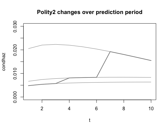
Lastly, here is an example that shows that the predictions respond now only over changing t values, but also to shifts in the time-varying covariate over the prediction period:

# Same model, but now look at a single time-varying covariate that changes over time
df2 <- df
df2$polity2 <- c(5, 5, 5, 3, 3, 3, -4, -4, -4, -4)

# add some hypothetical lines for constant polity2 values to highlight the shifts 
plot(1:10, seq(0, .03, length.out = 10), type = "n", xlab = "t", ylab = "condhaz")
df_i <- df2
for (p2 in c(5, 3, -4)) {
  df_i$polity2 <- p2
  condhaz_i <- predict(model.coups2, newdata = df_i)
  lines(1:10, condhaz_i, col = "gray50")
}

condhaz <- predict(model.coups2, newdata = df2)
lines(1:10, condhaz, col = "gray50", lwd = 2)
title(main = "Polity2 changes over prediction period")

Answer 2

My experience is that in general, time varying covariates is implemented & used with little thought and elegance (because the simplest method works ok!).

The canonical method is to simply use regular regresion-fitting algos but letting data for each timestep and subject be a row in the dataset.

You have to go pretty deep into an absurd frequentist rabbit hole to get this to fit into the rest of regression-puritan theory, and I dont personally grasp why this is legal in most cases but heck - it works. I think this is the reason why you can't find in depth discussions or implementations of it. Thinking about it spoils the fun!

If you want to be fancy about it (I would) I'd add survival time (known at prediction time so ok feature) as a variable.

The next is something i like to do but not sure about how common it is. I'd also weight each observation s.t:

1. Rows contribute according to how long they would be used i.e time to next datapoint (s.t sum weights per subject proportional to survival time for that subject) . This counters high frequency time-clustered observations getting undue influence. Permits loss to be interpreted as 'time that we're correct'

2. Rows for each subject contribute equally. (Weights per subject sum to 1) Counters that subjects with many observations gets undue influence.