Tips and tricks for getting good parameter estimates using Bayesian nonlinear regression

Question

I've been playing around with fitting nonlinear models using rjags. Specifically 3 and 4 parameter sigmoid curves, e.g.,

upAsym + (y0 - upAsym)/ (1 + (x[r]/midPoint)^slope))

I've noticed that good parameter estimates (+- 95% HDIs) are highly dependent upon having tightly constrained priors. Are there any good guidelines (or easy read papers/books) that can help with choosing reasonable uninformative priors to aid parameter estimation?

I'm thinking along the lines of: whether it's better to have uniform priors over a specific range vs using moderate precision normal priors, or, fitting a least squares estimate first to help set boundaries and starting values, or, adjust the burn in and thinning.

A toy example I've been playing with (the slope parameter in this example can sometimes be difficult to get a decent estimate for):

x <- 0:20
y <- 20 + (2 - 20)/(1 + (x/10)^5) + rnorm(21, sd=2)
dataList = list(y = y, x = x, N = 21)

models = "
model {
  for( i in 1 : N ) {
    y[i] ~ dnorm( mu[i] , tau )
    mu[i] <- upAsym + (y0 - upAsym)/ (1 + pow(x[i]/midPoint, slope))
  }
  tau ~ dgamma( sG , rG )
  sG <- pow(m,2)/pow(d,2)
  rG <- m/pow(d,2)
  m ~ dgamma(1, 0.01)
  d ~ dgamma(1, 0.01)

  midPoint ~ dnorm(10,0.0001) T(0,21)
  slope    ~ dnorm(5, 0.0001) T(0,)
  upAsym   ~ dnorm(30,0.0001) T(0,40)
  y0       ~ dnorm(0, 0.0001) T(-20,20)
}" 
writeLines(models,con="model.txt")

Answer 1

Here's the notation I'm going to use for the sigmoid model:

$y = U + \frac{L - U}{1 + (\frac{x}{x_0})^k}$

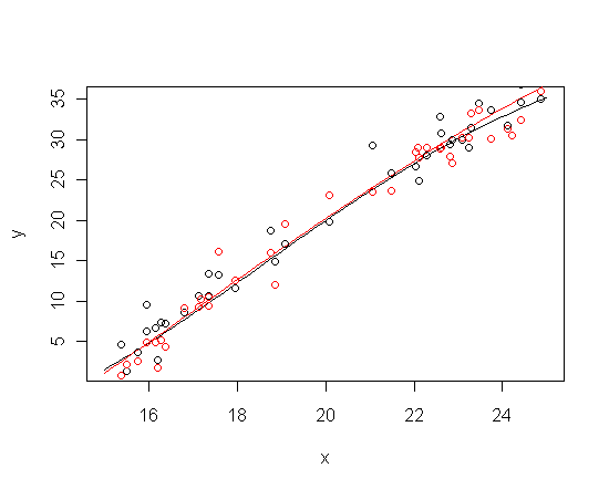
The problem is that the sigmoid model nests functions that are close to linear within a bounded domain, and further, that very different parameter values give rise to almost-lines that are almost the same. Check it out:

sigmoid <- function(x, L, U, x_0, k) U + (L-U)/(1 + (x/x_0)^k)
x<- runif(n = 40, min = 15, max = 25)
y1 <- sigmoid(x, -10, 50, 20, 5) + rnorm(length(x), sd = 2)
y2 <- sigmoid(x, -24, 76, 21.6, 3) + rnorm(length(x), sd = 2)
curve(sigmoid(x, -10, 50, 20, 5), from = 15, to = 25, ylab = "y")
curve(sigmoid(x, -24, 76, 21.6, 3), add = TRUE, col = "red")
points(x, y1)
points(x, y2, col = "red")

The upshot is that the likelihood function changes very, very slowly in some directions over vast swaths of the parameter space. If the priors don't constrain the parameters, then the posterior distribution inherits the likelihood's ill-conditioning.

I haven't used jags, so I don't know how much freedom you have to specify priors. (When things get this complicated I usually roll my own sampling algorithm in R.) The approach I'd use in this situation is to give zero prior support to sigmoid functions that don't have detectable saturation on both ends of the data domain (by "data domain" I mean the closed interval between the minimum and maximum $x$ values). This won't work unless the data really do turn out to have detectable saturation at both ends -- but if the data look linear on either end, one shouldn't be fitting a sigmoid anyway.

First, note that slope of the function at the midpoint is $\frac{(U-L)k} {4x_0}$. Let the set of $x$ values for which the ratio of slope of the sigmoid function to the slope at the midpoint is at most $\frac{1}{2}$ be the "saturation regions". There will be two saturation regions, one above the midpoint and one below. Points in these regions contribute most of their information to determining the values of the asymptotes. In fact, estimating an asymptote is basically like estimating a constant, so the standard error of the estimate of an asymptote is approximately $\frac{\sigma}{\sqrt{n}}$, where $n$ is the number of data points in the appropriate saturation region.

Let $n_U$ and $n_L$ be the number of data points within the upper and lower saturation regions, respectively. Note that these numbers are implicitly functions of all the parameters of the sigmoid function. To exclude regions of flat likelihood from the prior support, I would choose a prior which assigns zero density unless the following conditions are satisfied:

• $x_0$ is within the data domain
• $n_U > 0$
• $n_L > 0$
• conditionally on $\sigma$, $U - \frac{2\sigma}{\sqrt{n_U}} > L + \frac{2\sigma}{\sqrt{n_L}}$

I'm not sure what prior is reasonable to assign within this region of prior support, but if it's just flat, at least it can't be worse than frequentist inference based on asymptotics of the likelihood function.