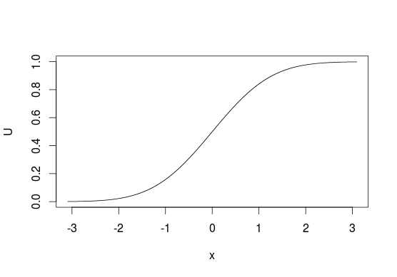
The method is very simple, so I'll describe it in simple words. First, take cumulative distribution function $F_X$ of some distribution that you want to sample from. The function takes as input some value $x$ and tells you what is the probability of obtaining $X \leq x$. So
$$ F_X(x) = \Pr(X \leq x) = p $$
inverse of such function function, $F_X^{-1}$ would take $p$ as input and return $x$. Notice that $p$'s are uniformly distributed -- this could be used for sampling from any $F_X$ if you know $F_X^{-1}$. The method is called the inverse transform sampling. The idea is very simple: it is easy to sample values uniformly from $U(0, 1)$, so if you want to sample from some $F_X$, just take values $u \sim U(0, 1)$ and pass $u$ through $F_X^{-1}$ to obtain $x$'s
$$ F_X^{-1}(u) = x $$
or in R (for normal distribution)
U <- runif(1e6)
X <- qnorm(U)
To visualize it look at CDF below, generally, we think of distributions in terms of looking at $y$-axis for probabilities of values from $x$-axis. With this sampling method we do the opposite and start with "probabilities" and use them to pick the values that are related to them. With discrete distributions you treat $U$ as a line from $0$ to $1$ and assign values based on where does some point $u$ lie on this line (e.g. $0$ if $0 \leq u < 0.5$ or $1$ if $0.5 \leq u \leq 1$ for sampling from $\mathrm{Bernoulli}(0.5)$).

Unfortunately, this is not always possible since not every function has its inverse, e.g. you cannot use this method with bivariate distributions. It also does not have to be the most efficient method in all situations, in many cases better algorithms exist.
You also ask what is the distribution of $F_X^{-1}(u)$. Since $F_X^{-1}$ is an inverse of $F_X$, then $F_X(F_X^{-1}(u)) = u$ and $F_X^{-1}(F_X(x)) = x$, so yes, values obtained using such method have the same distribution as $X$. You can check this by a simple simulation
U <- runif(1e6)
all.equal(pnorm(qnorm(U)), U)

