Solving log-logistic distribution parameters from moments

Question

Let's say we have a log-logistic random variable $X$ with probability density function:

$$f(x)=\frac{(\beta/\alpha)(x/\alpha)^{\beta-1}}{(1+(x/\alpha)^{\beta})^{2}}$$

where $\alpha>0$, $\beta>0$ and support on $x\in[0,\infty)$.

This random variable has mean and variance defined as follows:

$$\mathbb{E}[X]=\frac{\alpha(\pi/\beta)}{\text{sin}(\pi/\beta)}$$ $$\text{Var}[X]=\alpha^{2}\bigg[\frac{2(\pi/\beta)}{\text{sin}(2(\pi/\beta))}-\frac{(\pi/\beta)^{2}}{\text{sin}^{2}(\pi/\beta)}\bigg]$$

or, more generally, with $k$th raw moment defined for $k<\beta$: $$\mathbb{E}[X^{k}]=\alpha^{k}\frac{k(\pi/\beta)}{\text{sin}(k\pi/\beta)}$$

Now, is there an clever way to estimate the parameters $(\alpha,\beta)$ such that it provides a desired mean and variance?

As far as I can tell, we can arrive at an equation in terms of either parameter, but solving requires some form of optimization. I was curious to know if there are any methods to avoid such optimization?

Answer 1

Note that $E(X^k)$ has $\alpha$ present only as a multiplicative term in $\alpha^k$.

As a result $E(X^a)^b/[E(X^b)^a]$ is a function of $\beta$ alone. Since $E(X^k)$ only exists for $\beta>k$ it's best to use lowest moments.

In particular, $E(X^2)/(E(X)^2)$ or $\operatorname{Var}(X)/(E(X)^2)$ or convenient functions of them may be used to solve for $\beta$ (at least numerically). Once $\beta$ is known, it is simple to obtain $\alpha$ from $E(X)$.

Now let's look at some convenient ways to obtain $\beta$.

Note that $\frac{2\sin^2(x)}{\sin(2 x)} = \frac{2\sin^2(x)}{2\sin(x)\cos(x)}= \tan(x)$ (on $0<x<\pi/2$).

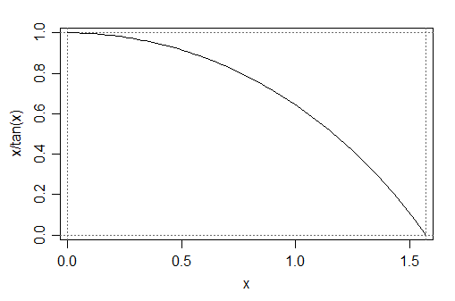
Let $\theta=\pi/\beta$. Then $E(X)^2/E(X^2)=\theta/\tan(\theta)$ for $0<\theta<\pi/2$ is monotonic decreasing in $\theta$, and has the added benefit that the function is bounded in this range. This should be reasonably simple to solve for $\theta$ using standard numerical root finding methods. Because $E(X)^2/E(X^2)$ will always lie between $0$ and $1$, this should always yield a possible solution (one with $\beta>2$)

However, we can get very close to to the solution -- and have bounds on it -- with just a little more manipulation.

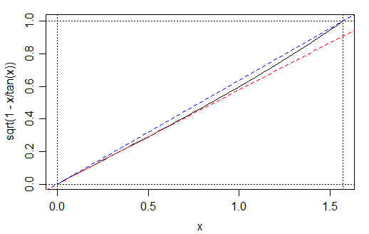
Note that $\sqrt{1-\frac{x}{\tan(x)}}$ is very close to linear:

In that interval it is bounded between the lines $x/\sqrt{3}$ and $\frac{2x}{\pi}$ -- which slopes only differ by about 10%.

So the steps would be:

• Compute $k=\sqrt{\frac{\sigma^2}{\sigma^2+\mu^2}}$.

• Solve the equation $\sqrt{1-\frac{\theta}{\tan(\theta)}}-k=0$ for $\theta$ via a convenient root-finding algorithm, with initial bounds $\frac{\pi}{2}k<\theta<\sqrt{3}k$. This should be very rapid.

• Obtain $\beta=\pi/\theta$

• Calculate $\alpha=\mu\frac{\sin\theta}{\theta}$.

Example: Let's say we want to figure out the parameters of a log-logistic distribution that would have $\mu=10$ and $\sigma=10$.

Then $k=\sqrt{\frac{10^2}{10^2+10^2}}=\sqrt{2}$. Using R:

f=function(x,k) {sqrt(1-x/tan(x))-k}
mu=10
sigma=10
k=sqrt(sigma^2/(sigma^2+mu^2))
f0 = uniroot(f,lower=k*pi/2,upper=min(pi/2,k*sqrt(3)),k=k)
f0
$root
[1] 1.165561

$f.root
[1] -3.517283e-08

$iter
[1] 3

$init.it
[1] NA

$estim.prec
[1] 6.103516e-05

So $\theta\approx 1.165561$.

 theta=f0$root
 beta=pi/theta
 alpha=10*sin(theta)/theta
 alpha;beta
[1] 7.884698
[1] 2.695348

Now let's check we actually got the mean and sd we were aiming for:

 alpha*pi/beta/sin(pi/beta)
[1] 10
 alpha*sqrt(2*pi/beta/sin(2*pi/beta)-(pi/beta)^2/sin(pi/beta)^2)
[1] 9.999999

About 7 digits of accuracy that time (we were probably a bit lucky getting the root quite so close to 0 that time; the estimated precision suggests it should not have worked quite that well).

Looks good; it seems to be doing what it should.