I often see people (statisticians and practitioners) transforming variables without a second thought. I've always been scared of transformations, because I worry they could modify the error distribution and thus lead to invalid inference, but it's so common that I have to be misunderstanding something.
To fix ideas, suppose I have a model
$$Y=\beta_0\exp X^{\beta_1}+\epsilon,\ \epsilon\sim\mathcal{N}(0,\sigma^2)$$
This could in principle be fit by NLS. However, nearly always I see people taking logs, and fitting
$$\log{Y}=\log\beta_0+\beta_1\log{X}+???\Rightarrow Z=\alpha_0+\beta_1W+???$$
I know this can be fitted by OLS, but I don't know how to compute the confidence intervals on the parameters, now, let alone prediction intervals or tolerance intervals.
And that was a very simple case: consider this considerably more complex (for me) case in which I don't assume the form of the relationship between $Y$ and $X$ a priori, but I try to infer it from data, with, e.g., a GAM. Let's consider the following data:
library(readr)
library(dplyr)
library(ggplot2)

# data
device <- structure(list(Amplification = c(1.00644, 1.00861, 1.00936, 1.00944,
1.01111, 1.01291, 1.01369, 1.01552, 1.01963, 1.02396, 1.03016,
1.03911, 1.04861, 1.0753, 1.11572, 1.1728, 1.2512, 1.35919, 1.50447,
1.69446, 1.94737, 2.26728, 2.66248, 3.14672, 3.74638, 4.48604,
5.40735, 6.56322, 8.01865, 9.8788, 12.2692, 15.3878, 19.535,
20.5192, 21.5678, 22.6852, 23.8745, 25.1438, 26.5022, 27.9537,
29.5101, 31.184, 32.9943, 34.9456, 37.0535, 39.325, 41.7975,
44.5037, 47.466, 50.7181, 54.2794, 58.2247, 62.6346, 67.5392,
73.0477, 79.2657, 86.3285, 94.4213, 103.781, 114.723, 127.637,
143.129, 162.01, 185.551, 215.704, 255.635, 310.876, 392.231,
523.313, 768.967, 1388.19, 4882.47), Voltage = c(34.7732, 24.7936,
39.7788, 44.7776, 49.7758, 54.7784, 64.778, 74.775, 79.7739,
84.7738, 89.7723, 94.772, 99.772, 109.774, 119.777, 129.784,
139.789, 149.79, 159.784, 169.772, 179.758, 189.749, 199.743,
209.736, 219.749, 229.755, 239.762, 249.766, 259.771, 269.775,
279.778, 289.781, 299.783, 301.783, 303.782, 305.781, 307.781,
309.781, 311.781, 313.781, 315.78, 317.781, 319.78, 321.78, 323.78,
325.78, 327.779, 329.78, 331.78, 333.781, 335.773, 337.774, 339.781,
341.783, 343.783, 345.783, 347.783, 349.785, 351.785, 353.786,
355.786, 357.787, 359.786, 361.787, 363.787, 365.788, 367.79,
369.792, 371.792, 373.794, 375.797, 377.8)), .Names = c("Amplification",
"Voltage"), row.names = c(NA, -72L), class = "data.frame")
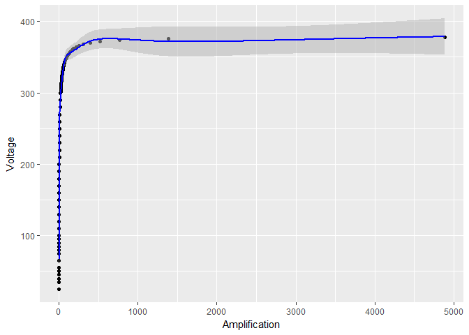
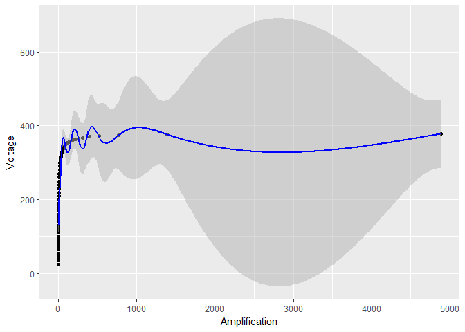
If I plot the data without log-transforming $X$, the resulting model and the confidence bounds don't look so nice:
# build model
model <- gam(Voltage ~ s(Amplification, sp = 0.001), data = device)

# compute predictions with standard errors and rename columns to make plotting simpler
Amplifications <- data.frame(Amplification = seq(min(APD_data$Amplification),
                                           max(APD_data$Amplification), length.out = 500))
predictions <- predict.gam(model, Amplifications, se.fit = TRUE)
predictions <- cbind(Amplifications, predictions)
predictions <- rename(predictions, Voltage = fit)

# plot data, model and standard errors
ggplot(device, aes(x = Amplification, y = Voltage)) +
  geom_point() +
  geom_ribbon(data = predictions,
              aes(ymin = Voltage - 1.96*se.fit, ymax = Voltage + 1.96*se.fit),
              fill = "grey70", alpha = 0.5) +
  geom_line(data = predictions, color = "blue")
But if I log-transform only $X$, it seems like the confidence bounds on $Y$ become much smaller:
log_model <- gam(Voltage ~ s(log(Amplification)), data = device)
# the rest of the code stays the same, except for log_model in place of model
 Clearly something fishy is going on. Are these confidence intervals reliable?
EDIT this is not simply a problem of the degree of smoothing, as it was suggested in an answer. Without the log-transform, the smoothing parameter is
> model$sp
s(Amplification)
     5.03049e-07
With the log-transform, the smoothing parameter is indeed much bigger:
>log_model$sp
s(log(Amplification))
         0.0005156608
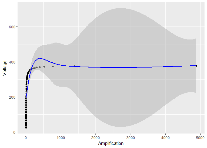
But this is not the reason why the confidence intervals become so small. As a matter of fact, using an even bigger smoothing parameter sp = 0.001, but avoiding any log-transform, oscillations are reduced (as in the log-transform case) but the standard errors are still huge with respect to the log-transform case:
smooth_model <- gam(Voltage ~ s(Amplification, sp = 0.001), data = device)
# the rest of the code stays the same, except for smooth_model in place of model
In general, if I log transform $X$ and/or $Y$, what happens to the confidence intervals? If it's not possible to answer quantitatively in the general case, I will accept an answer which is quantitative (i.e., it shows a formula) for the first case (the exponential model) and gives at least an hand-waving argument for the second case (GAM model).


mgcvcan be represented as a sum of terms of the type $x^2\log(x)$ - I may try them. What's Voung's test? Can you provide more details? Do you know if it's implemented in a R package? $\endgroup$