How to interpret Lasso shrinking all coefficients to 0?

Question

I've got a dataset with 338 predictors and 570 instances (can't upload unfortunately) on which I'm using the Lasso to perform feature selection. In particular, I'm using the cv.glmnet function from glmnet as follows, where mydata_matrix is a 570 x 339 binary matrix and the output is binary too:

library(glmnet)
x_dat <- mydata_matrix[, -ncol(mydata_matrix)]
y <- mydata_matrix[, ncol(mydata_matrix)]
cvfit <- cv.glmnet(x_dat, y, family='binomial')

This plot shows that the lowest deviance occurs when all variables have been removed from the model. Is this really saying that just using the intercept is more predictive of the outcome than using even a single predictor, or have I made a mistake, possibly in the data or in the function call?

This is similar to a previous question, but that didn't get any responses.

plot(cvfit)

Answer 1

I don't think you have made a mistake in the code. This is a matter of interpreting the output.

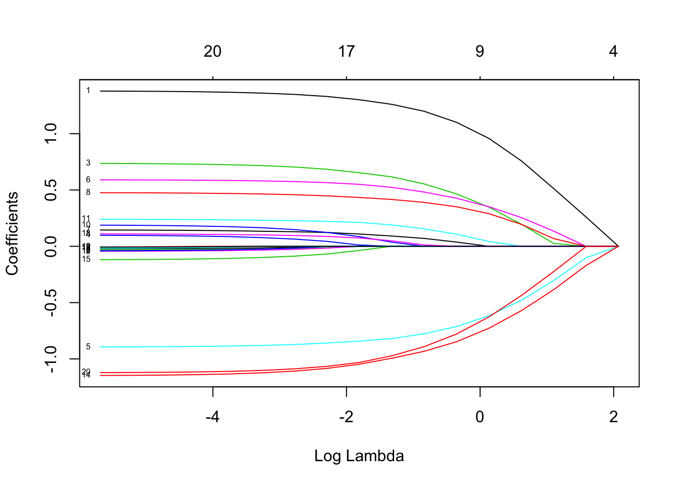
The Lasso doesn't indicate which individual regressors are "more predictive" than others. It simply has a built-in tendency to estimate coefficients as zero. The larger the penalty coefficient $\log(\lambda)$ is, the greater is that tendency.

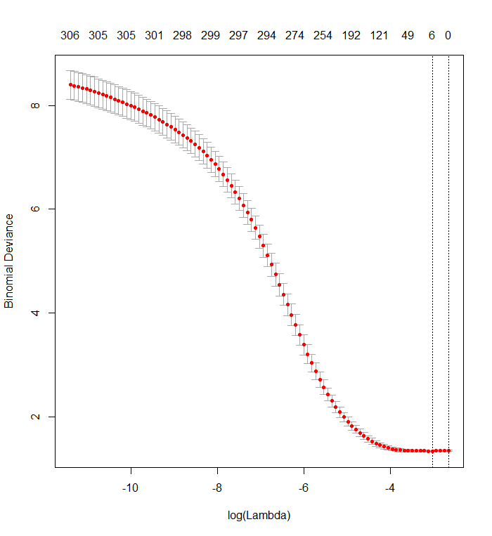
Your cross-validation plot shows that as more and more coefficients are forced to zero, the model does a better and better job of predicting subsets of values that have been randomly removed from the dataset. When the best cross-validated prediction errors (measured as the "Binomial Deviance" here) are achieved when all coefficients are zero, you should suspect that no linear combination of any subset of the regressors may be useful for predicting the outcomes.

You can verify this by generating random responses that are independent of all the regressors and applying your fitting procedure to them. Here's a quick way to emulate your dataset:

n <- 570
k <- 338
set.seed(17)
X <- data.frame(matrix(floor(runif(n*(k+1), 0, 2)), nrow=n,
                       dimnames=list(1:n, c("y", paste0("x", 1:k)))))

The data frame X has one random binary column named "y" and 338 other binary columns (whose names don't matter). I used your approach to regress "y" against those variables, but--just to be careful--I made sure the response vector y and model matrix x match up (which they might not do in case there are any missing values in the data):

f <- y ~ . - 1            # cv.glmnet will include its own intercept
M <- model.frame(f, X)
x <- model.matrix(f, M)
y <- model.extract(M, "response")
fit <- cv.glmnet(x, y, family="binomial")

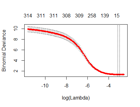
The result is remarkably like yours:

plot(fit)

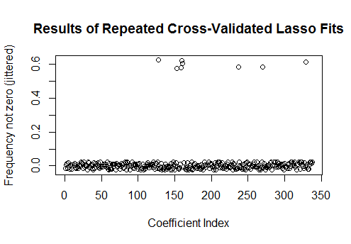
Indeed, with these completely random data the Lasso still returns nine nonzero coefficient estimates (even though we know, by construction, that the correct values are all zero). But we shouldn't expect perfection. Moreover, because the fitting is based on randomly removing subsets of the data for cross-validation, you typically won't get the same output from one run to the next. In this example, a second call to cv.glmnet produces a fit with only one nonzero coefficient. For this reason, if you have the time, it's always a good idea to re-run the fitting procedure several times and keep track of which coefficient estimates are consistently nonzero. For these data--with hundreds of regressors--this will take a couple of minutes to repeat nine more times.

sim <- cbind(as.numeric(coef(fit)), 
             replicate(9, as.numeric(coef(cv.glmnet(x, y, family="binomial")))))
plot(1:k, rowMeans(sim[-1,] != 0) + runif(k, -0.025, 0.025), 
     xlab="Coefficient Index", ylab="Frequency not zero (jittered)",
     main="Results of Repeated Cross-Validated Lasso Fits")

Eight of these regressors have nonzero estimates in about half of the fits; the rest of them never have nonzero estimates. This shows to what extent the Lasso will still include nonzero coefficient estimates even when the coefficients themselves are truly zero.

Answer 2

If you want to obtain more informations can use the function

fit1<-glmnet(x_dat, y, family='binomial', alpha= x)

plot(fit1, xvar = "lambda", label = TRUE)

The graph should be similar to The labels allow to identify the effect of lambda for the regressors.

Can you use differents value of x ( in the model is called alpha factor) to 0 (ridge regression) to 1 (LASSO Regression). The value [0,1] are the elastic net regression

Answer 3

It's possible but a little surprising. LASSO can do weird things when you have collinearity, in which case you should probably set alpha<1 so you're fitting elastic net instead. You can choose alpha by cross-validation but make sure you're using the same folds for each value of alpha.

Answer 4

The answer that there are no linear combinations of variables that are useful in predicting outcomes is true in some but not all cases.

I had a plot like the one above which was caused by multicollinearity in my data. Reducing the correlations allowed Lasso to work but it also removed useful information about the outcomes. Better sets of variables were obtained by using random forest importance to screen variables and then using Lasso.

Answer 5

One possible reason is that the classes are imbalanced in your train and val datasets. Try stratifed sampling to split the whole dataset into train and val subsets. That is, make the event ratios same between train and val.