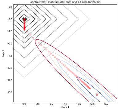
As has been pointed out by others, Lasso can set coefficients to zero, thus in essence excluding them from the model. (Technically, the coefficient still affects the model since its initial inclusion affects how the other variables' coefficients are shrunk. More on this shrinkage soon.)
Furthermore, even when the coefficients are not set to zero, they tend to be shrunk towards zero. This can be seen by looking at what the ordinary least squares (OLS) estimated coefficients have minimized and compare it to the Lasso solution. In the notation below, $\beta=\beta_1, \ldots, \beta_p$ is a vector of $p$ coefficients, $\beta_0$ is an intercept, $y_i$ is the outcome of individual $i=1,\ldots,n$ and $x_{ki}$ is the value of covariate $k=1,\ldots,p$ for individual $i$.
$\hat{\beta}^{OLS} = \underset{\beta}{\arg\min}\left\{\underset{i=1}{\overset{n}{\sum}}\left( y_i - \beta_0 - \underset{k=1}{\overset{p}{\sum}}\beta_k x_{ki}\right)^2 \right\}$
That is, the OLS solution tries to minimize the mean squared error of prediction of $y_i$. If the covariates are highly correlated, it is known that this can lead to very instable estimates of the corresponding $\beta_k$. This high variance of the estimates can lead to $\beta_k$ to often be estimated far too large (in either direction). To combat that, the Lasso solution finds the solution that minimizes the mean squared error, penalized by the sum of the absolute value of the estimated coefficients.
$\hat{\beta}^{Lasso} = \underset{\beta}{\arg\min}\left\{\underset{i=1}{\overset{n}{\sum}}\left( y_i - \beta_0 - \underset{k=1}{\overset{p}{\sum}}\beta_k x_{ki}\right)^2 + \lambda \underset{k=1}{\overset{p}{\sum}} \vert\beta_k\vert \right\}$, for some $\lambda \geq 0.$
This means that solutions that have high values of the estimated coefficients are not as often selected as they would be in the OLS case. This leads to less variance in the estimated coefficients.
The cost of this adjustment is bias, as while $E\left(\hat{\beta}^{OLS}\right)=\beta$ even in the presence of multicollinearity, $E\left(\hat{\beta}^{Lasso}\right)\neq\beta$. Thus the choice of using the Lasso over OLS follows the usual bias-variance trade-off.
To summarize, the aspect of multicollinearity that Lasso combats is the high variance of the estimated coefficients that results from multicollinearity. It does this by shrinking coefficients towards zero, reducing the variance but introducing bias. Furthermore, it can set coefficients to exactly zero. This is unlike the very related Ridge regression (Hoerl & Kennard, 1970), where the coefficients are shrunk but can't be set to zero.
If you want more details about Lasso, Ridge and similar shrinkage techniques, I recommend Hastie et al. (2009).
References:
Hastie, T., Tibshirani, R., and Friedman, J. (2009). The elements of statistical learning. Springer series in statistics. Springer, New York, 11th printing, 2nd edition.
Hoerl, A. E., and Kennard, R. W. (1970). Ridge regression: Biased estimation for nonorthogonal problems. Technometrics, 12(1), 55-67.

