The dirty coins and the three judges

Question

All things being perfect, if we want to know if a set of coinage (all coins with the same bias) is biased, and to what degree, we would just use the outcomes and confidence intervals of the binomial distribution and be done with it.

Unfortunately, things are rarely that simple in real life. Indeed, this question arose as one of my concerns for what seems like a completely different problem elsewhere. If we are not sure what the true outcome is, and we have to adjudicate the results, that muddies the waters, and alters the confidence interval width. Now suppose we have dirty coins and we do not know for sure what is a heads or tails, or, some other similar problem, like having to use adjudication with three judges to say which image reconstruction method is more diagnostic (for example), then how well the judges agree with each other becomes a factor in whether we can detect that one method of image reconstruction is better than another or whether we can detect biased coinage.

Question: How do we determine, without having truth data, how sloppy our confidence interval is if we have three judges who do not always agree with each other as to what the outcome is?

Now, I did not know how to calculate this (but see answer below after help from colleagues), but I could simulate it, and even the simulation has a curve ball. To that in a minute, first though, keep in mind that we do not have access to the hidden truth in the real world, all we know is probable truth. However, we can assign a synthetic truth when we simulate results.

The simulation

I did 10,000 binary random trials with 3 different biases of coinage, 0.5, (0.2, 0.8), and (0.1 0.9). Note that a bias of p=0.2 is symmetric with p=0.8, so that the 3 trials covers 5 cases in total. Next, as I had that as truth data, I could arbitrarily assign known reliabilities for our judges, and for each judge I simulated their decisions using two factors. For example, for a reliability (or correct knowledge, if you will) of 50%, I allowed the truth data to influence that judges decision 50% of the time. The next factor is that I randomized the remaining decisions, i.e., 50% in our example to be a yes 50% of the time (the latter is perfect cluelessness). That means that for a reliability of 50%, the judge will make a correct decision a factor of 0.5 + 0.5 p of the time. However, to increase the overall reliability of adjudication, we need more than one judge.

Now the curve ball. With three judges, I was able to contrast two strategies to adjudicate their decisions. These are 1) The median result, which is appealing because it is always a 0,1; yes or no, or 2) the mean result. Now let is look at the result for 10,000 trials of three adjudications each.

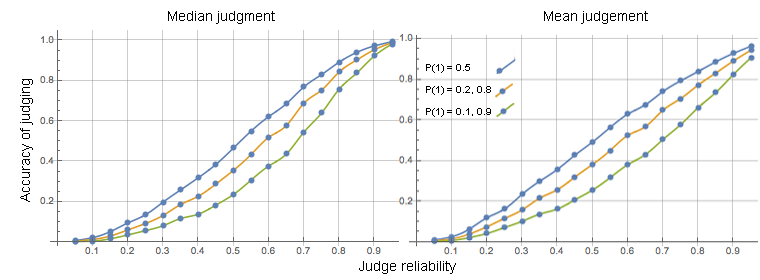
In the figure, the $y$-axis represents R$^2$, i.e., explained fraction, and the $x$-axis represents the judges reliability. Note that the most accurate (i.e., efficient) results were had when coinage was 50-50 (p=0.5). However, that is also the least useful result in the sense of being able to detect the one method is better than the other for image reconstruction or for detecting coinage bias. When the three judges' reliability was >0.63, the median method outperformed the mean as an adjudication strategy. This became pronounced when the judges were very reliable (0.95). On the other hand, the mean became the better adjudication strategy for more unreliable judging (<0.63). Now results for single judges are not shown, they were miserable.

In the real world case, the judges might have different abilities, one might be 50% reliable and another 80%, depending on how 'expert' they are. Notwithstanding, for the real case, we only need some indication as to how to calculate our confidence intervals more or less accurately, and any insight into this interesting problem would be welcome.

Answer 1

If you rephrase the question,

• not asking about the 'true' $p_{coin}$ how often the coin is heads or tails
• but instead you analyze the 'effective' $p_{judges}$ the probability how often the judges say heads or tails

, then the regular analysis becomes 'ok'.

This analysis does not become more difficult. Even if the $p_{judges}$ is not a constant like $p_{coin}$ (the probability that the judges say heads or tails is not a constant every throw); the distribution of the outcome can still be modeled as a Bernoulli distribution (a mixture of Bernoulli distributions is a Bernoulli distribution).

---

The outcomes from the three judges together could possibly be modeled as a beta-binomial distribution, or one could throw other more specific analyses at it. But this depends on assumptions that we can make about the consistency and variability among judges. at least we can do more than the simple Bernoulli distribution.

For instance: in the case of the dirty coins we should expect some correlation between the occasions that the judges make false/random judgments. We can expect that, if we split the judges results into unanimous and non-unanimous, then the $p$ obtained from these different groups could differ. This allows us to make estimates about $p_{coin}$ based on the two versions of $p_{judges}$. (without such analysis then we only know that $|p_{coin}-0.5| \geq |p_{judges}-0.5|$ but we do not know by how much without a good guess of the reliability)

Answer 2

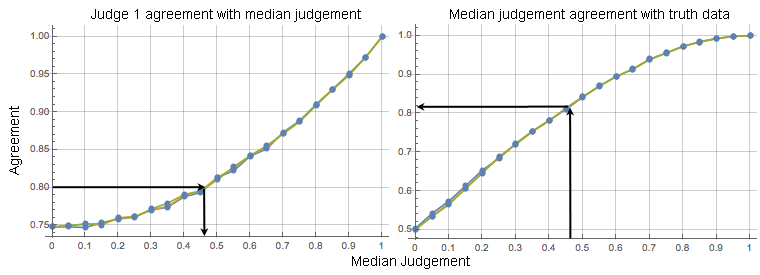
The problem simplifies if we quantify agreement, where by agreement we mean the fraction of $0$'s and $1$'s of the total number of trials that are the same between any two measurements. In specific, we quantify how each (equally good) judge’s judgments agree with the median judgments, and how well median judgements agree with the truth data, as below.

First note that each panel above represents 3 curves, and they superimpose. Those curves represents 5 different biases of coinage, $0.5, (0.2, 0.8),$ and $(0.1, 0.9)$. Thus, we have eliminated (apart from noise) the effect of bias on the measurements in a way that cannot be had from correlation. This occurs because agreement of a $0$ with a $0$ is as useful as agreement of a $1$ with a $1$. Thus, it does not matter what the relative number of $1$'s and $0$'s is, just whether those outcomes are the same or different for a single judge and the median judgments.

To use these curves, we calculate the agreement of one of the judges with the median judgments using available data. We then use the curves to back solve for the median judgments. That curve appears to be from total probability $\text{J}1_{\text{agr}}=\dfrac{3}{4}+\dfrac{\text{M}^{2}}{4}$, whose back solution is $\text{M}=\sqrt{4 \,\text{J}1_{\text{agr}}-3}$. We know from simulation that a particular value of median judgments corresponds to a unique (or nearly so) fraction of agreement with the truth data. This appears to be also from total probability $\text{Agr(frac)}=-\dfrac{\text{M}^3}{4}+\dfrac{3 \text{M}}{4}+\dfrac{1}{2}$. That value, in turn, times the $n$ trials, gives us a number of agreements. It is that number, $<n$, which is the basis for calculating confidence intervals. As that number is less than the number of trials, our confidence intervals will be different. As we shall see in a bit, how they differ depends on judge training. To complete our analysis, we need to make a further assumption and that is that an adequately trained judge makes unbiased errors of judgment. That is, his errors of judgment are $0$’s and $1$’s 50% of the time.

Suppose that there were $60$ yes’s (e.g., Yes, picture A is more diagnostic than picture B) and $40$ no’s with an agreement fraction of $0.8$. Then we write $60-x+40-x=80$, or $x=10$ giving us a truth value of $50$ yes’s and $30$ no’s in our “truth” population of $100\times0.8=80$. Then $P$(yes)$=\frac{50}{80}=0.625$, which finally gives us enough information to calculate confidence intervals. The 95% CI for our $50$ out of $80$ yes's was $40.92119$ to $57.83999$, and does not include $40$, where $40$ or $\dfrac{1}{2}$ of the $80$ results would be $p=0.0151145$ one-tailed. Note, as the binomial distribution only allows for whole numbers, I calculated the CI's using the binomial CDF real number equivalent $I_{1-p}(n-k,k+1)$, i.e., the regularized beta function of those parameters.

If we had used the original number of trials in our example; $100$, with a median judgement of $60$ yes's, our one-tailed $p(k\leq 50)$ would be $0.0270992$, and two-tails would have been $p>0.05$. So, it can make a difference how we calculate this. Moreover, training makes a difference. Untrained judgements may have errors in proportion to voting numbers, e.g., $60x+40x=80\rightarrow48$ yes votes out of $80$ [$p(k\leq40)=0.0444971$, one-tailed] and not $50/80,\,p(k\leq40)=0.0151145$ one-tailed. Even that may underestimate the effect of a lack of training, because the agreement of an untrained judge with the median may be worse as well. What is training? For example, for adjudicating diagnostic images, one either knows what all of the applicable diagnoses are, or the judgment is uninformed. That is, the training either covers off all possible implications or we are better off not using that judgement, at least in those circumstances where the outcome really needs adjudication, i.e., is not immediately obvious. So, we saw that the confidence intervals were relatively more narrow for trained judges than for the uncorrected problem, which, in turn, had a relatively smaller confidence interval than that for the corrected results for untrained judges, that is, for our single example case.

The polynomials used fit the above curves well, $r\sim 0.9999$ for median judgments agreement with truth data, and $\sim 0.9997$ for single judge agreement with the median judgment. The former was suggested by a linear transform of a sigmoidal-like smoothstep functional relationship with the data. The latter appears to be a simple probability calculation. Since we can test for each judge's results compared to the median, and the percentage of yes's and no's, it may be possible to extend the analysis here to include judges of unequal talent, contrarian judges who vote the opposite of what they actually think, and maybe even somewhat for biased judging, or at least we can test for the presence/absence of biased decision making among judges.