Data cleansing in regression analysis

Question

I've got a dataset for Temperature & KwH and I'm currently performing the regression below. (further regression based on coeffs is performed within PHP)

# Some kind of List structure..
UsageDataFrame  <- data.frame(Energy, Temperatures);

# lm is used to fit linear models. It can be used to carry out regression,
# single stratum analysis of variance and analysis of covariance (although
# aov may provide a more convenient interface for these).
LinearModel     <- lm(Energy ~ 1+Temperatures+I(Temperatures^2), data = UsageDataFrame)

# coefficients
Coefficients    <- coefficients(LinearModel)

system('clear');

cat("--- Coefficients ---\n");
print(Coefficients);
cat('\n\n');

The issue comes with our data, we can't ensure there isn't random communication failures or just random errors. This can leave us with values like

Temperatures <- c(16,15,13,18,20,17,20);
Energy <- c(4,3,3,4,0,60,4)

Temperatures <- c(17,17,14,17,21,16,19);
Energy <- c(4,3,3,4,0,0,4)

Now as humans we can clearly see that the 60 for Kwh is a mistake based on the temperature, however we have over 2,000 systems each with multiple meters and each in different locations all over the country.. and with different levels of normal Energy usage.

A normal dataset would be 48 values for both Temperatures & Energy per day, per meter. In a full year its likely we could have around 0-500 bad points per meter out of 17520 points.

I've read other posts about the tawny package however I've not really seen any examples which would me to pass a data.frame and it process them through cross analysis.

I understand not much can be done, however big massive values surely could be stripped based on the temperature? And the number of times it occurs..

Since R is maths based I see no reason to move this into any other language.

Please note: I'm a Software Developer and have never used R before.

-- Edit --

Okay here's a real world example, seems this meter is a good example. You can see the Zeros are building up then a massive value is inserted. "23, 65, 22, 24" being examples of this. This happens when its in comms failure and it holds the data value and continues to add it up on the device.

(Just to say the comms failures are out of my hands nor can I change the software)

However because Zero is a valid value im wanting to remove any massive numbers against the temperatures or Zeros where its clear they are an Error.

The thought of detecting this and averaging the data back isn't a fix for this either, however it was discussed but since this meter data is every 30mins and comms failures can happen for days.

Most systems are using more Energy then this so its perhaps a bad example from a removing Zero's point of view.

Energy: http://pastebin.com/gBa8y5sM Temperatures: http://pastie.org/4371735

(Pastebin seems to have gone down for me after posting such a big file)

Answer 1

Use a robust fit, such as lmrob in the robustbase package. This particular one can automatically detect and downweight up to 50% of the data if they appear to be outlying.

To see what can be accomplished, let's simulate a nasty dataset with plenty of outliers in both the $x$ and $y$ variables:

library(robustbase)
set.seed(17)
n.points <- 17520
n.x.outliers <- 500
n.y.outliers <- 500
beta <- c(50, .3, -.05)
x <- rnorm(n.points)
y <- beta[1] + beta[2]*x + beta[3]*x^2 + rnorm(n.points, sd=0.5)
y[1:n.y.outliers] <- rnorm(n.y.outliers, sd=5) + y[1:n.y.outliers]
x[sample(1:n.points, n.x.outliers)] <- rnorm(n.x.outliers, sd=10)

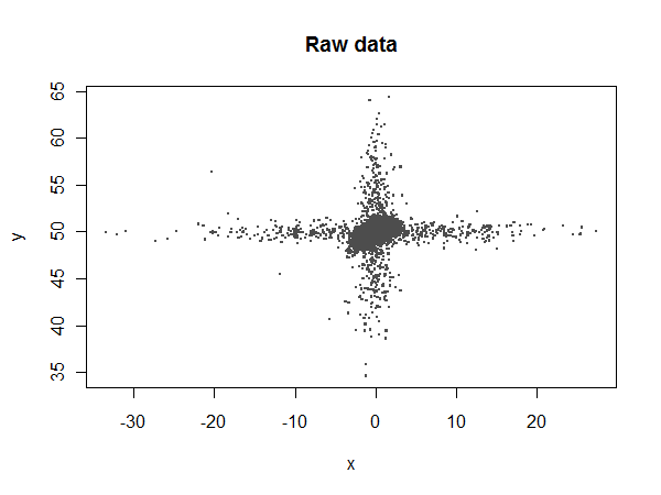
Most of the $x$ values should lie between $-4$ and $4$, but there are some extreme outliers:

Let's compare ordinary least squares (lm) to the robust coefficients:

summary(fit<-lm(y ~ 1 + x + I(x^2)))
summary(fit.rob<-lmrob(y ~ 1 + x + I(x^2)))

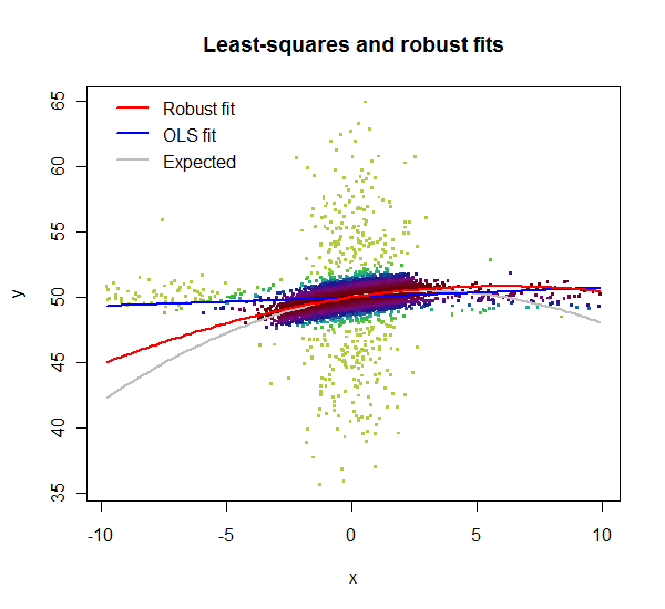
lm reports fitted coefficients of $49.94$, $0.00805$, and $0.000479$, compared to the expected values of $50$, $0.3$, and $-0.05$. lmrob reports $49.97$, $0.274$, and $-0.0229$, respectively. Neither of them estimates the quadratic term accurately (because it makes a small contribution and is swamped by the noise), but lmrob comes up with a reasonable estimate of the linear term while lm doesn't even come close.

Let's take a closer look:

i <- abs(x) < 10        # Window the data from x = -10 to 10
w <- fit.rob$weights[i] # Extract the robust weights (each between 0 and 1)
plot(x[i], y[i], pch=".", cex=4, col=hsv((w + 1/4)*4/5, w/3+2/3, 0.8*(1-w/2)), 
     main="Least-squares and robust fits", xlab="x", ylab="y")

lmrob reports weights for the data. Here, in this zoomed-in plot, the weights are shown by color: light greens for highly downweighted values, dark maroons for values with full weights. Clearly the lm fit is poor: the $x$ outliers have too much influence. Although its quadratic term is a poor estimate, the lmrob fit nevertheless closely follows the correct curve throughout the range of the good data ($x$ between $-4$ and $4$).