1
$\begingroup$

I have some count data pertaining to number of events observed among independent trials in 3 groups of an experiment:

count   A    B    C
0       5    0    5
1       1   25    9
2       9   30   10
3       3   15    8
4       4   13    9
5       4   13    5
6       1    6    8
7       2    4    6
8       0   10    1
9       4    5    2
10      0    5    3

A Kruskal-Wallis test leads me to conclude that the distribution of numbers of events observed does not differ significantly between groups. However, I'd also like to know whether getting a specific event count is statistically more likely in the different groups. In particular I'm interested in event counts of zero or 1. For example, an event count of 1 is proportionately much more likely in group B compared with groups A or C. I'd like to test for the significance of this.

I have looked at using a chi-squared test to compare proportions between groups for a specific outcome but believe this may be invalid due to low frequencies of observation (<5) for some numbers of events. In this case, would R's prop.test be more suitable?

EDIT: post updated to make data easy to copy-and-paste

$\endgroup$
13
  • 1
    $\begingroup$ Could you show your data in a form suitable for copy-and-paste? Presenting tables as images cuts down mightily on the number of people who might play with your data to give other perspectives. $\endgroup$
    – Nick Cox
    Apr 18, 2018 at 16:38
  • 1
    $\begingroup$ (Previous comment deleted). For what you are asking, I think one approach is to construct a 2 x 3 table of counts with e.g. "1" and "Not-1" for A, B, and C. You could run a chi-square test or Fisher's exact on that table.... But looking at your data, it seems strange that you want to look at only, say, counts for "1" events. Is there something special about "1" vs. "2" or "0" relative to the rest? $\endgroup$ Apr 18, 2018 at 17:30
  • 1
    $\begingroup$ I think your instinct to use Kruskal-Wallis was a good one. But comparing the distributions with a chi-square test of association on the whole table may also make sense. The expected counts for the whole table are pretty small. (Maybe 15% are less than 2). So you might want to use an exact test (fisher.test) or Monte Carlo: library(coin); chisq_test(Table, distribution=approximate(B=100000)). For a visual: library(lattice); histogram(~Counts.f | Group, data = All, layout = c(1,3), col="gray") $\endgroup$ Apr 18, 2018 at 18:30
  • 1
    $\begingroup$ @allhands, your confusion stems from the fact that you have the hypothesis for the K-W test incorrect. Unfortunately people have the tendency --- either being sloppy or trying to simplify things --- to say that Wilcoxon-Mann-Whitney and K-W test the distribution of the data in the groups. This is misleading. They test the probability that an observation from one group will be higher in rank than from another group. The null is stochastic equality among the groups. Practically, they test if one group has higher values than another, not if the distributions differ in some other way. $\endgroup$ Apr 19, 2018 at 13:24
  • 1
    $\begingroup$ For post-hoc, sometimes people look at standardized residuals or odds ratio. For me, the most logical way to is break down the table pairwise. In this case, you would construct a table with A and B, one with A and C, and one with B and C. Be sure to apply a p-value correction for multiple tests. There are some functions used here that automate this process. As mentioned above, if you are looking specifically at, say, a count of "1", you can construct a 2x3 table of counts for "1" and "not-1". Again, be aware that you are making multiple hyp tests. $\endgroup$ Apr 19, 2018 at 14:09

2 Answers 2

1
$\begingroup$

I can't reproduce your chi-square result. This is what I get in Stata:

          observed frequency
          expected frequency

----------------------------------
          |         which         
    count |      A       B       C
----------+-----------------------
        0 |      5       0       5
          |  1.467   5.600   2.933
          | 
        1 |      1      25       9
          |  5.133  19.600  10.267
          | 
        2 |      9      30      10
          |  7.187  27.440  14.373
          | 
        3 |      3      15       8
          |  3.813  14.560   7.627
          | 
        4 |      4      13       9
          |  3.813  14.560   7.627
          | 
        5 |      4      13       5
          |  3.227  12.320   6.453
          | 
        6 |      1       6       8
          |  2.200   8.400   4.400
          | 
        7 |      2       4       6
          |  1.760   6.720   3.520
          | 
        8 |      0      10       1
          |  1.613   6.160   3.227
          | 
        9 |      4       5       2
          |  1.613   6.160   3.227
          | 
       10 |      0       5       3
          |  1.173   4.480   2.347
----------------------------------

16 cells with expected frequency < 5

          Pearson chi2(20) =  42.0876   Pr = 0.003
 likelihood-ratio chi2(20) =  47.3624   Pr = 0.001

We can note:

  1. Strong rejection of lack of association. Plainly put, the groups really are different.

  2. Caveat: several small expected frequencies.

  3. Caveat: The chi-square test pays no attention to the ordering 0 ... 10 or what those values are. They are just 11 categories.

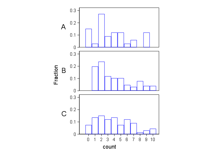
The distributions do look different.

enter image description here

I can't comment helpfully on the idea of focusing on 0 and 1. I am not a routine user of R and haven't looked at prop.test, but note that it is best to phrase questions in terms of statistical issues, not the software you happen to be using.

$\endgroup$
11
  • $\begingroup$ Thanks for this. Your chi-square output is the same, in that we reject independence of the variables (event count and group), i.e. there is some association between them. But the Kruskal-Wallis result indicates that we cannot reject the null hypothesis that the samples are from the same distribution. So on one hand chi-square says there is an effect between group and event count, but on the other KW says they are not different. Am I mis-interpreting something here? $\endgroup$
    – allhands
    Apr 19, 2018 at 11:34
  • $\begingroup$ The "prop.test" function tests whether proportions between groups are the same. To run this I believe the data would need to be mapped as "success" and "failure", or "event count = 1" vs. "event count != 1" in my example. $\endgroup$
    – allhands
    Apr 19, 2018 at 11:35
  • 2
    $\begingroup$ For the Monte Carlo (coin :: chisq_test), I got (approximately) chi-squared = 42.088, p-value = 0.00259, just about the same as the usual chi-squared test. $\endgroup$ Apr 19, 2018 at 14:17
  • 2
    $\begingroup$ @SalMangiafico That's fine and I'm just showing fewer d.p. on the P-value. OP's different results remain. $\endgroup$
    – Nick Cox
    Apr 19, 2018 at 14:26
  • 1
    $\begingroup$ In short, small expected frequencies aren't biting: I suggested earlier that they have to really small for that to happen. The P-value is trustworthy and its implications clear. If you want to follow up the issue of small counts @SalMangiafico has made specific suggestions. under the question. $\endgroup$
    – Nick Cox
    Apr 19, 2018 at 14:41
0
$\begingroup$

You are mainly interested in knowing how to interpret the test results when there are more than two categories. Particularly, as you stated: "I would like to know whether getting a specific event count is statistically more likely in the different groups"

Therefore, I am sharing a brief script that I use in such situations:

# Load the required packages:
library(MASS) # for chisq
library(descr) # for crosstable

CrossTable(a$exam_result, a$ethnicity
       fisher = T, chisq = T, expected = T,
       prop.c = F, prop.t = F, prop.chisq = F, 
       sresid = T, format = 'SPSS')

This code will generate both Pearson's Chi-square and Fisher's Chi square. It produces counts as well as proportions of each of the table entries. Based on the standardised residuals or z-values scores i.e.,

sresid

For each table entry, look at its sresid, whenever it is outside the range |1.96| i.e., less than -1.96 or greater than 1.96, then it is significant p < 0.05. And its sign would then indicate whether it is positively related or negatively.

$\endgroup$

Your Answer

By clicking “Post Your Answer”, you agree to our terms of service and acknowledge you have read our privacy policy.

Not the answer you're looking for? Browse other questions tagged or ask your own question.