Fitting a distribution to match known points on the CDF

Question

I've recently run into a situation where I know a few probability points in the tail of a distribution and I want to "fit" a distribution that goes through these points in the tail. I realize this is messy and not overly accurate, and plagued with conceptual issues. However, trust me that I really want to do this.

So effectively I know some points in the tail of the CDF with x being the values and y being the probability of that value or smaller. Here's R code to illustrate my data:

x <- c(0.55, 0.6, 0.65, 0.7, 0.75, 0.8, 0.85)
y <- c(0.0666666666666667, 0.0625, 0.0659340659340659, 0.0563106796116505, 
       0.0305676855895196, 0.0436953807740325, 0.0267459138187221)

Then I create a function to minimize error between my data and a beta distribution CDF using pbeta. I use SSE as a fit metric then minimize that with -sum. I throw in an initial guess as the first param to optim of (9, .8) although I've tried this with different guesses and I always get the same result. The starting point guess I use comes from manually cooking up parameters by hand that seem close.

# function to optomize with optim
beta_func <- function(par, x) -sum( (pbeta( x, par[1], par[2]) - y)**2 ) 
out <- optim(c(9,.8), beta_func, lower=c(1,.5), upper=c(200,200), method="L-BFGS-B", x=x)

out <- out$par
print(out)
#> [1]  0.90000 23.40294

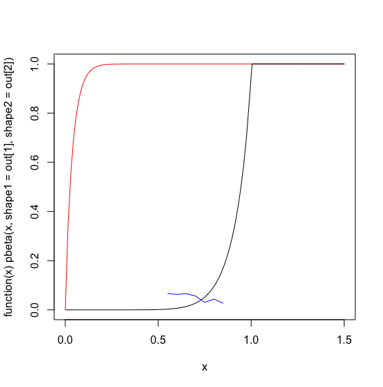
Below I graph the 'optimized' beta distribution in red, my actual data in blue, and a hand tweaked starting guess of the beta parameters in black.

plot(function(x) pbeta(x, shape1=out[1], shape2=out[2] ), 0, 1.5, col='red')
plot(function(x) pbeta(x, 9,.8), 0, 1.5, col='black', add=TRUE)
lines(x,y, col='blue')

I can't grok what's going on with optim to give a solution that's worse than my starting guess. I calculated the SSE for my starting guess vs the optim solution and it looks like my guess has a much larger -SSE:

# my guess
-sum( (pbeta( x, 9, .8) - y)**2)
#> [1] -0.03493344

# optim's output
-sum( (pbeta( x, .9, 23) - y)**2)
#> [1] -6.314587

Using past history as my Bayesian prior, my guess is that I'm misunderstanding optim or feeding it improper inputs. However, I can't grok what's going on. Any tips would be greatly appreciated.

I've tried using the CG optimization method, but the results are not meaningfully different and still don't seem near as good as my starting guess.

out <- optim(c(9,.8), beta_func, method="CG", x=x)
out <- out$par
print(out)
#> [1]  2.287611 11.124736

Answer 1

I think you are accidentally trying to maximize the squared errors. The default for optim() is to minimize the function, so the negative sign in your beta_func() results in searching for a max.

If you modify your function like so you get values closer to your guess:

beta_func2 <- function(par, x) sum( (pbeta( x, par[1], par[2]) - y)**2 ) 
out2 <- optim(c(9,.8), beta_func2, lower=c(1,.5), upper=c(200,200), method="L-BFGS-B", x=x)
out2 <- out2$par
print(out2)
[1] 11.04296  0.50000

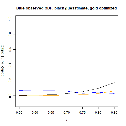
You can check the new function against your observations (where out, x, and y are defined as in your example):

plot(x,(pbeta(x,out[1],out[2])), ylim=c(-.1,1), col="red", type="l")
points(x, (pbeta(x,9,0.8)), col="black", type="l")
points(x,(pbeta(x,out2[1],out2[2])), col="orange", type="l")
lines(x,y, col='blue')
title(main="Blue observed CDF, black guesstimate, gold optimized")