25
$\begingroup$

I have read the most popular books in statistical learning

1- The elements of statistical learning.

2- An introduction to statistical learning.

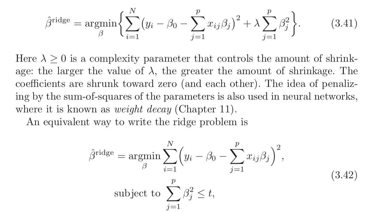
Both mention that ridge regression has two formulas that are equivalent. Is there an understandable mathematical proof of this result?

I also went through Cross Validated, but I can not find a definite proof there.

Furthermore, will LASSO enjoy the same type of proof?

enter image description here

$\endgroup$
7
  • 2
    $\begingroup$ en.wikipedia.org/wiki/… $\endgroup$
    – Taylor
    Commented May 27, 2018 at 18:56
  • 1
    $\begingroup$ Lasso is not a form of ridge regression. $\endgroup$
    – Xi'an
    Commented May 28, 2018 at 17:10
  • $\begingroup$ @jeza, Could you explain what's missing in my answer? It really derives all can be derived about the connection. $\endgroup$
    – Royi
    Commented May 30, 2018 at 20:13
  • $\begingroup$ @jeza, Could you be specific? Unless you know the Lagrangian concept for constrained problem it is hard to give a concise answer. $\endgroup$
    – Royi
    Commented May 31, 2018 at 4:34
  • 1
    $\begingroup$ @jeza , a constrained optimization problem can be converted into optimization of the Lagrangian function / KKT conditions (as explained in the current answers). This principle has already many different simple explanations all over the internet. In what direction is more explanation of the proof necessary? Explanation/proof of the Lagrangian multiplier/function, explanation/proof how this problem is a case of optimization that relates to the method of Lagrange, difference KKT/Lagrange, explanation of the principle of regularization, etc? $\endgroup$ Commented May 31, 2018 at 7:05

4 Answers 4

23
$\begingroup$

The classic Ridge Regression (Tikhonov Regularization) is given by:

$$ \arg \min_{x} \frac{1}{2} {\left\| x - y \right\|}_{2}^{2} + \lambda {\left\| x \right\|}_{2}^{2} $$

The claim above is that the following problem is equivalent:

$$\begin{align*} \arg \min_{x} \quad & \frac{1}{2} {\left\| x - y \right\|}_{2}^{2} \\ \text{subject to} \quad & {\left\| x \right\|}_{2}^{2} \leq t \end{align*}$$

Let's define $ \hat{x} $ as the optimal solution of the first problem and $ \tilde{x} $ as the optimal solution of the second problem.

The claim of equivalence means that $ \forall t, \: \exists \lambda \geq 0 : \hat{x} = \tilde{x} $.
Namely you can always have a pair of $ t $ and $ \lambda \geq 0 $ such the solution of the problem is the same.

How could we find a pair?
Well, by solving the problems and looking at the properties of the solution.
Both problems are Convex and smooth so it should make things simpler.

The solution for the first problem is given at the point the gradient vanishes which means:

$$ \hat{x} - y + 2 \lambda \hat{x} = 0 $$

The KKT Conditions of the second problem states:

$$ \tilde{x} - y + 2 \mu \tilde{x} = 0 $$

and

$$ \mu \left( {\left\| \tilde{x} \right\|}_{2}^{2} - t \right) = 0 $$

The last equation suggests that either $ \mu = 0 $ or $ {\left\| \tilde{x} \right\|}_{2}^{2} = t $.

Pay attention that the 2 base equations are equivalent.
Namely if $ \hat{x} = \tilde{x} $ and $ \mu = \lambda $ both equations hold.

So it means that in case $ {\left\| y \right\|}_{2}^{2} \leq t $ one must set $ \mu = 0 $ which means that for $ t $ large enough in order for both to be equivalent one must set $ \lambda = 0 $.

On the other case one should find $ \mu $ where:

$$ {y}^{t} \left( I + 2 \mu I \right)^{-1} \left( I + 2 \mu I \right)^{-1} y = t $$

This is basically when $ {\left\| \tilde{x} \right\|}_{2}^{2} = t $

Once you find that $ \mu $ the solutions will collide.

Regarding the $ {L}_{1} $ (LASSO) case, well, it works with the same idea.
The only difference is we don't have closed for solution hence deriving the connection is trickier.

Have a look at my answer at StackExchange Cross Validated Q291962 and StackExchange Signal Processing Q21730 - Significance of $ \lambda $ in Basis Pursuit.

Remark
What's actually happening?
In both problems, $ x $ tries to be as close as possible to $ y $.
In the first case, $ x = y $ will vanish the first term (The $ {L}_{2} $ distance) and in the second case it will make the objective function vanish.
The difference is that in the first case one must balance $ {L}_{2} $ Norm of $ x $. As $ \lambda $ gets higher the balance means you should make $ x $ smaller.
In the second case there is a wall, you bring $ x $ closer and closer to $ y $ until you hit the wall which is the constraint on its Norm (By $ t $).
If the wall is far enough (High value of $ t $) and enough depends on the norm of $ y $ then i has no meaning, just like $ \lambda $ is relevant only of its value multiplied by the norm of $ y $ starts to be meaningful.
The exact connection is by the Lagrangian stated above.

Resources

I found this paper today (03/04/2019):

$\endgroup$
22
  • 1
    $\begingroup$ @jeza, As I wrote above, for any $ t $ there is $ \lambda \geq 0 $ (Not necessarily equal to $ t $ but a function of $ t $ and the data $ y $) such that the solutions of the two forms are the same. $\endgroup$
    – Royi
    Commented May 28, 2018 at 4:07
  • 4
    $\begingroup$ @jeza, both $\lambda$ & $t$ are essentially free parameters here. Once you specify, say, $\lambda$, that yields a specific optimal solution. But $t$ remains a free parameter. So at this point the claim is that there can be some value of $t$ that would yield the same optimal solution. There are essentially no constraints on what that $t$ must be; it's not like it has to be some fixed function of $\lambda$, like $t=\lambda/2$ or something. $\endgroup$ Commented May 29, 2018 at 20:46
  • 1
    $\begingroup$ @Royi, I have a few things. 1- what do you mean by "move form my 𝜆 to the OP 𝜆 by a factor of two. 2" not clear to me yet. 2- I am still cannot understand that logic. 3- I am confused because you introduce "mu" with "t" and "lambda", also "‖𝑦‖^2_2≤𝑡 one must set 𝜇=0 which means that for 𝑡 large enough in order for both to be equivalent one must set 𝜆=0. 𝑦𝑡(𝐼+2𝜇𝐼)−1(𝐼+2𝜇𝐼)−1𝑦=𝑡. This is basically when ‖𝑥̃ ‖22=𝑡" not clear to me. 4- I expect to see that "t" = "lambda" then you mentioned "mu" = "lambda". Could you please help me by elaborating or editing the answer. Thx $\endgroup$
    – jeza
    Commented Apr 2, 2019 at 23:17
  • 1
    $\begingroup$ @Royi, I think the question will be duplicated! $\endgroup$
    – jeza
    Commented Apr 4, 2019 at 10:14
  • 2
    $\begingroup$ The most confusing part is that the relation between $\lambda$ and $t$ is data-dependent. @Royi has mentioned this twice in the comments, but IMO this is an important point that deserves to be put in bold in the answer. Although this fact is somewhat obvious (for given $\lambda, t$ we scale $y$ away from the regression line, so that the solution penalised by $\lambda$ doesn't fit into the constraint set by $t$), the phrasing "equivalent way to write the problem" is misleading, as in order to write the problem in the equivalent way we are required to first solve it. $\endgroup$ Commented May 10, 2022 at 23:58
13
+25
$\begingroup$

A less mathematically rigorous, but possibly more intuitive, approach to understanding what is going on is to start with the constraint version (equation 3.42 in the question) and solve it using the methods of "Lagrange Multiplier" (https://en.wikipedia.org/wiki/Lagrange_multiplier or your favorite multivariable calculus text). Just remember that in calculus $x$ is the vector of variables, but in our case $x$ is constant and $\beta$ is the variable vector. Once you apply the Lagrange multiplier technique you end up with the first equation (3.41) (after throwing away the extra $-\lambda t$ which is constant relative to the minimization and can be ignored).

This also shows that this works for lasso and other constraints.

$\endgroup$
3
  • 2
    $\begingroup$ Don’t we have to treat it as Karush-Kuhn-Tucker rather than Lagrange, since the constraint is an inequality? $\endgroup$
    – Dave
    Commented Sep 24, 2020 at 11:44
  • $\begingroup$ @Dave, Would this make any real difference? (It has been quite a while since I was in a calculus class and don't remember the details of how they compare). From a practical standpoint (understanding rather than rigorous proof), any meaningful constraints considered will have the solution equal to the constraint, so I don't think it will really matter. $\endgroup$
    – Greg Snow
    Commented Sep 24, 2020 at 13:38
  • $\begingroup$ @Dave even if you take the KKT formulation, your lambda hyperparameter is positive, which means all the KKT inequality constraints are activ, i.e. they are on the boundary g(x)=0. This comes down to the Lagrangian formulation because we only have equality constraints left. $\endgroup$
    – Matt
    Commented Aug 21, 2021 at 12:23
13
$\begingroup$

It's perhaps worth reading about Lagrangian duality and a broader relation (at times equivalence) between:

  • optimization subject to hard (i.e. inviolable) constraints
  • optimization with penalties for violating constraints.

Quick intro to weak duality and strong duality

Assume we have some function $f(x,y)$ of two variables. For any $\hat{x}$ and $\hat{y}$, we have:

$$ \min_x f(x, \hat{y}) \leq f(\hat{x}, \hat{y}) \leq \max_y f(\hat{x}, y)$$

Since that holds for any $\hat{x}$ and $\hat{y}$ it also holds that:

$$ \max_y \min_x f(x, y) \leq \min_x \max_y f(x, y)$$

This is known as weak duality. In certain circumstances, you have also have strong duality (also known as the saddle point property):

$$ \max_y \min_x f(x, y) = \min_x \max_y f(x, y)$$

When strong duality holds, solving $\max_y \min_x f(x, y)$ also solves $\min_x \max_y f(x, y)$.

Lagrangian for constrained Ridge Regression

Let me define the function $\mathcal{L}$ as:

$$ \mathcal{L}(\mathbf{b}, \lambda) = \sum_{i=1}^n (y - \mathbf{x}_i \cdot \mathbf{b})^2 + \lambda \left( \sum_{j=1}^p b_j^2 - t \right) $$

The min-max interpretation of the Lagrangian

The Ridge regression problem subject to hard constraints is:

$$ \min_\mathbf{b} \max_{\lambda \geq 0} \mathcal{L}(\mathbf{b}, \lambda) $$

You pick $\mathbf{b}$ to minimize the objective, cognizant that after you pick $\mathbf{b}$, your opponent will set $\lambda$ to infinity if you chose $\mathbf{b}$ such that the constraint was violated (in this case $\sum_{j=1}^p b_j^2 > t$).

If strong duality holds (which it does here because it's a convex optimization problem where Slater's condition is satisfied for $t>0$), you then achieve the same result by reversing the order:

$$ \max_{\lambda \geq 0} \min_\mathbf{b} \mathcal{L}(\mathbf{b}, \lambda) $$

In this dual problem, your opponent chooses $\lambda$ first! You then choose $\mathbf{b}$ to minimize the objective, already knowing your opponent's choice of $\lambda$. The $\min_\mathbf{b} \mathcal{L}(\mathbf{b}, \lambda)$ part (taking $\lambda$ as given) is equivalent to the 2nd form of your Ridge Regression problem.

As you can see, this isn't a result particular to Ridge Regression. It is a broader concept.

References

I started this post following an exposition of Rockafellar.

Rockafellar, R.T., Convex Analysis

You might also examine lectures 7 and lecture 8 from Prof. Stephen Boyd's course on convex optimization.

$\endgroup$
2
  • 1
    $\begingroup$ note that your answer can be extended to any convex function. $\endgroup$
    – 81235
    Commented Jul 8, 2019 at 16:07
  • $\begingroup$ In the maxmin formulation $\max_{\lambda \geq 0} \min_\mathbf{b} \mathcal{L}(\mathbf{b}, \lambda)$ shouldn't we maximize with respect to $\lambda$ (as we do in the Wolfe dual in SVM's) or is it because we select (we fix) the value of $\lambda$? $\endgroup$ Commented Jan 11, 2023 at 22:04
9
$\begingroup$

They are not equivalent.

For a constrained minimization problem

$$\min_{\mathbf b} \sum_{i=1}^n (y - \mathbf{x}'_i \cdot \mathbf{b})^2\\ s.t. \sum_{j=1}^p b_j^2 \leq t,\;\;\; \mathbf b = (b_1,...,b_p) \tag{1}$$

we solve by minimize over $\mathbf b$ the corresponding Lagrangean

$$\Lambda = \sum_{i=1}^n (y - \mathbf{x}'_i \cdot \mathbf{b})^2 + \lambda \left( \sum_{j=1}^p b_j^2 - t \right) \tag{2}$$

Here, $t$ is a bound given exogenously, $\lambda \geq 0$ is a Karush-Kuhn-Tucker non-negative multiplier, and both the beta vector and $\lambda$ are to be determined optimally through the minimization procedure given $t$.

Comparing $(2)$ and eq $(3.41)$ in the OP's post, it appears that the Ridge estimator can be obtained as the solution to

$$\min_{\mathbf b}\{\Lambda + \lambda t\} \tag{3}$$

Since in $(3)$ the function to be minimized appears to be the Lagrangean of the constrained minimization problem plus a term that does not involve $\mathbf b$, it would appear that indeed the two approaches are equivalent...

But this is not correct because in the Ridge regression we minimize over $\mathbf b$ given $\lambda >0$. But, in the lens of the constrained minimization problem, assuming $\lambda >0$ imposes the condition that the constraint is binding, i.e that

$$\sum_{j=1}^p (b^*_{j,ridge})^2 = t$$

The general constrained minimization problem allows for $\lambda = 0$ also, and essentially it is a formulation that includes as special cases the basic least-squares estimator ($\lambda ^*=0$) and the Ridge estimator ($\lambda^* >0$).

So the two formulation are not equivalent. Nevertheless, Matthew Gunn's post shows in another and very intuitive way how the two are very closely connected. But duality is not equivalence.

$\endgroup$
11
  • $\begingroup$ @MartijnWeterings Thanks for the comment, I have reworked my answer. $\endgroup$ Commented May 31, 2018 at 7:58
  • $\begingroup$ @MartijnWeterings I do not see what is confusing since the expression written in your comment is exactly the expression I wrote in my reworked post. $\endgroup$ Commented May 31, 2018 at 8:50
  • 2
    $\begingroup$ This was the duplicate question I had in mind were the equivalence is explained very intuitively to me math.stackexchange.com/a/336618/466748 the argument that you give for the two not being equivalent seems only secondary to me, and a matter of definition (the OP uses $\lambda \geq 0$ instead of $\lambda > 0$ and we could just as well add the constrain $t < \Vert \beta^{OLS} \Vert^2_2$ to exclude the cases where $\lambda=0$) . $\endgroup$ Commented May 31, 2018 at 9:38
  • 1
    $\begingroup$ @MartijnWeterings When A is a special case of B, A cannot be equivalent to B. And ridge regression is a special case of the general constrained minimization problem, Namely a situation to which we arrive if we constrain further the general problem (like you do in your last comment). $\endgroup$ Commented May 31, 2018 at 9:44
  • $\begingroup$ Certainly you could define some constrained minimization problem that is more general then ridge regression (like you can also define some regularization problem that is more general than ridge regression, e.g. negative ridge regression), but then the non-equivalence is due to the way that you define the problem and not due to the transformation from the constrained representation to the Lagrangian representation. The two forms can be seen as equivalent within the constrained formulation/definition (non-general) that are useful for ridge regression. $\endgroup$ Commented May 31, 2018 at 9:51

Your Answer

By clicking “Post Your Answer”, you agree to our terms of service and acknowledge you have read our privacy policy.

Not the answer you're looking for? Browse other questions tagged or ask your own question.