Indeed, the fractions of suicide $\frac{3}{83}$ and $\frac{0}{84}$ are different. That is correct. But for a good research report, we also want to express how much this observation may have been due to chance.
There are all sorts of ways to compare these numbers. To get these differences intuitively. Maybe it is more intuitive/straightforward to do some modeling/computing...
Probability of getting 0 cases
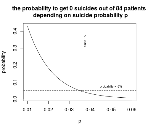
Let's consider the probability to get 0 cases out of 84 patients when the assumed suicide probability is $p$.
This is a binomial distribution, and the Poisson distribution is only an approximation of the binomial distribution.
Indeed the probability to get 0 or fewer suicides out of 84 when $p = 3/83$ is below 0.05
$$\begin{array}{rcl}
P(K \leq k | n,p) &=& \sum_{i=0}^k {n\choose i} p^{i}(1-p)^{n-i} \\
P(K \leq 0 | n=84, p = \frac{3}{83}) &\approx& 0.04539407
\end{array}$$
The curve below shows how this probability depends on $p$

### plot curve
p <- seq(0.01,0.06, 10^-4)
y <- dbinom(x = 0, size = 84, prob = p)
plot(p, y,main="the probability to get 0 suicides out of 84 patients \n depending on suicide probability p",
     type = "l", xlab = "p", ylab = "probability")

### plot lines and intercept
lines(c(1,1)*3/83,c(-10,10),lty=2)
text(0.036,0.38,"p = 3/83", col = 1, pos = 4, srt = -90, cex = 0.7)
lines(c(-1,1)*100,c(1,1)*0.05,lty=2)
text(0.05,0.05,"probabilty = 5%", col = 1, pos = 3, srt = 0, cex = 0.7)
points(3/83,dbinom(0,84,3/83), pch = 21, col = 1, bg = 0, cex =0.7)
Probability of opportunistic post-hoc comparison
You would assume that the null hypothesis is that the probability of suicide in both groups is the same: $p = p_1 = p_2$. The true suicide probability $p$ is unknown and this is what makes the analysis difficult.
In the study, the authors use one group as the reference and see whether, based on that one group, the other group is significantly different. But is that really significant?
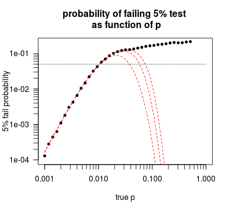
Let's try it out with a simulation of how often we would infer that the bigger group is significantly larger than the smaller group.
the simulation shows clearly that with this approach you do not really get a true p-value. Given the hypothesis $p = p_1 = p_2$ the probability to reject this hypothesis is not constant and equal to the p-value. What the researchers compute is a p-value based on the assumption that the result from the other group is correct. But this is not the probability that they find a discrepancy.

### function to perform simulation
### the value returned, nneg/N_trials
### is how often the null get's rejected
###
rate <- function(p, n1 =84, n2 = 83, N_trials = 10^5) {
  nneg <- 0 ### counters for how often the test fails

  for (i in 1:N_trials) {

    ###  simulate N_trials experiments
    x1 <- rbinom(1, size = n1, prob = p)
    x2 <- rbinom(1, size = n2, prob = p)
    p1 <- (x1/n1)
    p2 <- (x2/n2)

    ### perform test
    if (p1>p2) {
      test <- pbinom(x2,n2,p1)
    } else {
      test <- pbinom(x1,n1,p2)
    }

    ### add tp counter when negative test
    if (test <= 0.05) {
      nneg = nneg + 1
    }
  }
  return (nneg/N_trials)
}

### Vectrize the function
rate <- Vectorize(rate,vectorize.args = "p")


### perform computations
set.seed(1)
p <- p <- 0.001 * 2^seq(0,9,0.25)
pr <- rate(p)


### plot results
plot(p, pr ,
     main="probability of failing 5% test \n as function of p",
     xlab = "true p", ylab = "5% fail probability",
     cex = 0.7 , pch = 21, col = 1, bg = 1, log = "xy",
     xlim = c(0.001,1), ylim = c(0.0001,0.2), xaxt = "n", yaxt = "n"
)

### logarithmic axis labels
axis(1, at = 0.001*c(c(1:10),c(2:10)*10,c(2:10)*100), labels = rep("",28))
axis(1, at = 0.001*c(1,10,100,1000))
axis(2, at = 0.0001*c(c(1:10),c(2:10)*10,c(2:10)*100), labels = rep("",28))
axis(2, at = 0.0001*c(1,10,100,1000), las = 2)


### this is what we expected 0.05 probability
lines(c(10^-6,1),c(1,1)*0.05, lty =3)

### this is a computation of the simulated probability
lines(p, 2*((1-pbinom(2, 84, prob = p))*dbinom(0, 83, prob = p)) , col =2, lty = 2 )

lines(p, 2*((1-pbinom(2, 84, prob = p))*dbinom(0, 83, prob = p) +
              (1-pbinom(4, 84, prob = p))*dbinom(1, 83, prob = p)) , col =2, lty = 2 )

lines(p, 2*((1-pbinom(2, 84, prob = p))*dbinom(0, 83, prob = p) +
              (1-pbinom(4, 84, prob = p))*dbinom(1, 83, prob = p) +
              (1-pbinom(6, 84, prob = p))*dbinom(2, 83, prob = p)) , col =2, lty = 2 )
Intuitively we can understand why the the first part in the graph is much lower than 5%. The probability to reject the null hypothesis rises very fast. It is the probability to get the 0 cases in one group and 3 or more cases in the other group (this probability is much smaller than 5%). We have plotted this in the graph with a red curve (we have plotted 3 red curves, the others are including the cases '1 suicide in the one group and 5 or more in the other' plus ' 2 suicides in the one group and 7 or more in the other').
The reason why the second part in the graph is much higher than 5% is in part because the the situation is two sided. If the two groups are in reality equal then you get half the time the one group larger and the other time the other group larger. This increases the probability to find a significant difference by two. The other part of the reason is because the test performed (how does one group compare to the other) is not reflecting the hypothesis test (the two groups are the same). The computation of the p-value assumes that the one group is the reference but it does not take into account that the difference between the two groups may be due to the one group being occasionally higher while the is occasionally lower.
Sample distribution of results and $\chi^2$
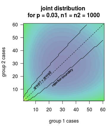
Below we plot the distribution of the results when the true suicide probability is 0.03 and the group sizes are 1000. For large group sizes, the distribution becomes more smooth/continuous and it can be approximated with a normal distribution.
You can see that for a given $p$ the distribution has some sort of spherical distribution. Getting further away from the line 'group1 = group2' is less likely. This is what the $\chi^2$ test measures. It looks how far we get from the line 'group1 = group2' and determines whether this is unlikely or not (we do not know what the true $p$ is and so we can not determine the p-value exactly, but we can use the estimated $p$ to determine this, or use the highest p-value out of all possible parameters $p$). The $\chi^2$ test does this by approximvting the distribution by a normal distribution.
(this works well with large numbers, and this is why I plotted the situation with large numbers, for your case with group size 84 and number of cases 3 the $\chi^2$ test is not accurate)
In the same plot I have plotted the rejection boundaries that relate to the article that you referenced. These types, of boundaries are not accurate because they only consider one of the two groups as variable and the other group is considered as the reference. This underestimates the variability in the difference between the two groups.

prob <- 0.03
n <- 1000

### generate joint distribution
x <- 1:61
y <- 1:61
z <- matrix(rep(0,61*61),61)
for (i in 1:61) {
  for(j in 1:61) {
    p <- dbinom(i,n,prob=prob)*dbinom(j,n,prob=prob)
    z[i,j] <- log(p)
  }
}

range(z)

# contour plot
filled.contour(x,y,z,
               xlab="group 1 cases",ylab="group 2 cases",
               #levels=c(-500,-400,-300,-200,-100,-10:-1),
               color.palette=function(n) {hsv(c(seq(0.15,0.7,length.out=n),0),
                                              c(seq(0.7,0.2,length.out=n),0),
                                              c(seq(1,0.7,length.out=n),0.9))},
               levels=seq(-60,0,2),
               plot.axes= c({
                 points(log(0.1+dat$action_count),log(2/3+dat$document_entropy))
                 points(log(0.1+dat$action_count)[which(dat$is_service == 1)],log(2/3+dat$document_entropy)[which(dat$is_service == 1)],pch=21,bg="red")
                 contour(x,y,z,add=1, levels=c(c(0:10)/10,10000))
                 title("joint distribution \n for p = 0.03, n1 = n2 = 1000 ")
                 axis(1)
                 axis(2)
                 lines(c(0,10^4),c(0,10^4), lty = 2)
                 text(15,17, "group1 = group2" ,srt = 45, cex = 0.7)
                 px <- 1:60
                 lines(px,qbinom(0.05,1000,px/1000))
                 lines(qbinom(0.05,1000,px/1000),px)
                 text(30,19, "rejection boundary" ,srt = 40, cex = 0.7)
               },""),
               xlim=range(x)+c(-0.05,0.05),
               ylim=range(y)+c(-0.05,0.05)
)
The bottom-line
The group sizes and the number of cases are too small to make reliable estimates.
The estimate they make is interresting but also slighlty optimistic. The above computations show how it is not a realistic p-value.
But, in addition, what we have not discusses above, the issue goes beyond the mathematics. The distribution of the test results is not a clean and nice binomial distribution (which is approximately Poisson distributed) and independent. The results might be biased which happens for instance when the experiment is not randomized or when the treatments are not blind. The test results migh be correlated, due to test procedures that are repeated within multiple subjects and not completely randomized. In this case the distributional assumptions are wrong (e.g. instead of i.i.d binomial distributed cases it might be including a random effect, or one might need to use a beta-binomial distribution instead).

