Background:
In community ecology one of the questions we are interested in is if the species in a community are non-randomly associated. To try and get at this we typically use a null modelling approach where we calculate an observed metric of association (co-occurrence) for the community. We then compare this observed value to the range of values obtained by shuffling the community matrix thousands of time.
You can then calculate a p-value based on how many of the values from the null distribution are greater or less than your observed value. You can also calculate a standardized effect size (SES) where SES = (observed value - mean of the null distribution)/standard deviation of the null distribution. The SES allows us to ask if the pattern of co-occurrence changes over time or if it is different from that of another community.
I generated several community matrices with only random patterns of association and I wanted to test and see if the null distributions for these communities are the same. My assumption being that if the distributions are not significantly different, then I can compare the observed metric of co-occurrence directly. To test this I used a meta-analysis (using the metafor package in R) providing the mean of the null distribution, the standard deviation and, the number of samples per study (the count of values in the null distribution) as input.
rma(mi = nullMean, sdi = nullStDev, ni = n, measure = "MN", method = "REML", data = DF)
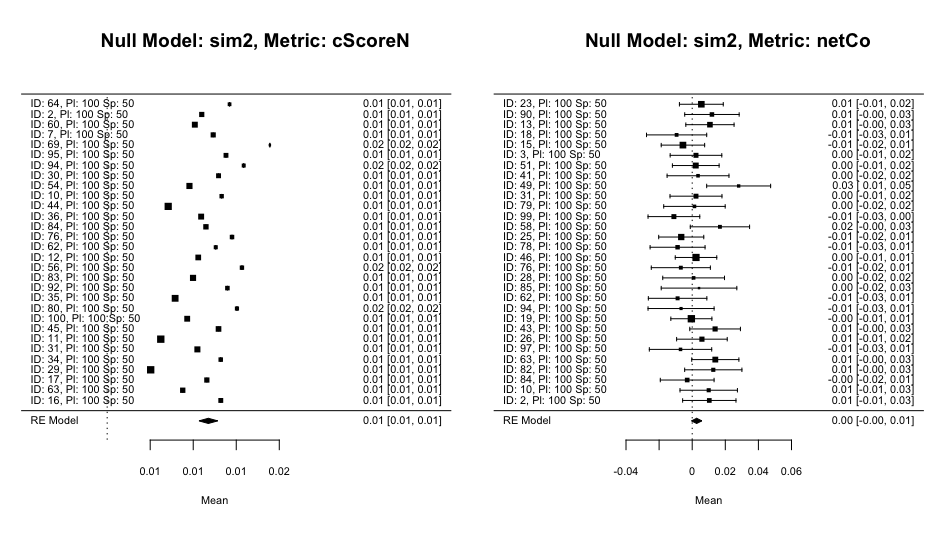
I did this for a couple of different metrics of association and using several null models. The plots and analyses output are examples of the two types of results I got.
[1] "#################################"
[1] "Null Model: sim2, Metric: cScoreN, SP: 50 Pl: 100"

Random-Effects Model (k = 30; tau^2 estimator: REML)

   logLik   deviance        AIC        BIC       AICc
 126.8605  -253.7211  -249.7211  -246.9865  -249.2596

tau^2 (estimated amount of total heterogeneity): 0.0000 (SE = 0.0000)
tau (square root of estimated tau^2 value):      0.0030
I^2 (total heterogeneity / total variability):   100.00%
H^2 (total variability / sampling variability):  299956.68

Test for Heterogeneity:
Q(df = 29) = 9857504.8837, p-val < .0001

Model Results:

estimate      se     zval    pval   ci.lb   ci.ub
  0.0118  0.0006  21.1286  <.0001  0.0107  0.0128  ***

---
Signif. codes:  0 ‘***’ 0.001 ‘**’ 0.01 ‘*’ 0.05 ‘.’ 0.1 ‘ ’ 1

[1] "#################################"
[1] "Null Model: sim2, Metric: netCo, SP: 50 Pl: 100"

Random-Effects Model (k = 30; tau^2 estimator: REML)

   logLik   deviance        AIC        BIC       AICc
  95.1906  -190.3812  -186.3812  -183.6466  -185.9196

tau^2 (estimated amount of total heterogeneity): 0.0000 (SE = 0.0000)
tau (square root of estimated tau^2 value):      0.0031
I^2 (total heterogeneity / total variability):   12.53%
H^2 (total variability / sampling variability):  1.14

Test for Heterogeneity:
Q(df = 29) = 34.3130, p-val = 0.2280

Model Results:

estimate      se    zval    pval    ci.lb   ci.ub
  0.0027  0.0016  1.6889  0.0912  -0.0004  0.0058  .

---
Signif. codes:  0 ‘***’ 0.001 ‘**’ 0.01 ‘*’ 0.05 ‘.’ 0.1 ‘ ’ 1
The results on the right are what I expected. The results on the left are what bring me to my question. Each study (matrix) on the left is significantly different from the overall result with no overlap of the confidence interval, the I^2 value is 100% and Q(df = 29) = 9857504.8837, p-val < .0001.
Given that each "study" is significantly different from the overall result (and from each other), is it valid to compare the SES values for the studies in the left hand plot to each other when the meta-analysis says they can not be combined and that they are measuring different effect?

