Based on @whuber's Comments about 'modeling', I gave some thought to relatively elementary methods that might be used to estimate the parameters of a normal distribution given the sample size, sample quartiles, and sample mean, assuming that data are normal.
Most of this will work better for very large $n.$ After some experimentation, I found that sample sizes around 35 are just large enough to get reasonably good results. All computations are done using R; seeds (based on current dates) are shown for simulations.
Hypothetical sample: So let's suppose we have a sample (rounded to two places) that is known to have come from a normal population of size
$n = 35,$ but with unknown $\mu$ and $\sigma.$ We are given that the sample mean is $A = 49.19,$ the sample median is $H = 47.72,$ and that the lower and upper quartiles are $Q_1 = 43.62,\, Q_3 = 54.73,$ respectively. (Sometimes reports and articles don't give complete datasets, but do give such summary data about the sample.)
Estimating the population mean. The best estimate of the population mean $\mu$ is the sample mean $A = \hat \mu = 49.19.$
Estimating the population standard deviation: If we knew it, a good estimate of the population standard deviation (SD) would be the sample SD $S,$ but that information is not given.
The interquartile range (IQR) of a standard normal population $1.35,$ and the IQR of a very large normal sample would be about $1.35\sigma.$
diff(qnorm(c(.25, .75)))
[1] 1.34898
set.seed(1018); IQR(rnorm(10^6))
[1] 1.351207
The IQR of our sample of size $n = 35$ is $54.73 - 43.62 = 11.11$ and the expected IQR of a standard normal sample of size 35 is 1.274. So we can estimate $\sigma$ for our population using the sample IQR: $\check \sigma = 11.11/1.274 = 8.72.$
set.seed(910);  m = 10^6;  n = 25
iqr = replicate(m, IQR(rnorm(n)))
mean(iqr);  sd(iqr)
[1] 1.274278
[1] 0.3024651
Assessing results: Thus, we can surmise that our normal population distribution is roughly,
$\mathsf{Norm}(49.19, 8.72).$ Actually, I simulated the sample from
$\mathsf{Norm}(50, 10).$
set.seed(2018);  x = round(rnorm(35, 50, 10), 2);  summary(x)
   Min. 1st Qu.  Median    Mean 3rd Qu.    Max.
  31.73   43.62   47.72   49.19   54.73   70.99
It seems worthwhile to make two comparisons: (a) how well does the given information match the CDF of $\mathsf{Norm}(49.19, 8.72),$ and (b) how well does the CDF of this estimated distribution match what we know to be the true normal distribution. Of course,
in a practical situation, we would not know the true normal distribution, so the second comparison would be impossible.
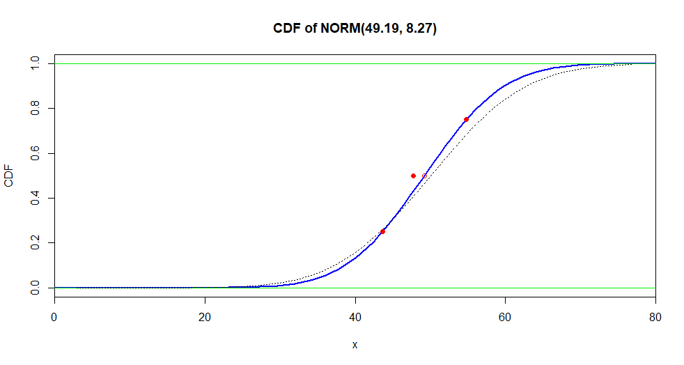
In the figure below, the blue curve is the estimated CDF; the solid red points show the sample values $Q_1, H, Q_3,$ and the red circle shows $A.$ The CDF of the true normal distribution is shown as a broken curve. It is no surprise that the three values $Q_1, Q_3,$ and $A$ used to estimate normal parameters fall near the estimated normal CDF.
curve(pnorm(x, 49.19, 8.27), 0, 80, lwd=2, ylab="CDF",
    main="CDF of NORM(49.19, 8.27)", xaxs="i", col="blue")
  abline(h=0:1, col="green2")
  points(c(43.62, 47.72, 54.73), c(.25, .5, .75), pch=19, col="red")
  curve(pnorm(x, 50, 10), add=T, lty="dotted")
  points(49.19, .50, col="red")

About symmetry: A remaining question is how much concern might have been appropriate about the normality of the data, upon noting that the sample mean exceeds the sample median by $D = A - H = 49.19 - 47.72 = 1.47.$
We can get a good idea by simulating the difference $D = A - H$ for many samples of size $n = 35$ from $\mathsf{Norm}(\mu = 49.19, \sigma = 8.27).$ A simple simulation shows that a larger positive difference might occur in such a normal sample about 11% of the time.
set.seed(918);  m = 10^6;  n = 25;  d = numeric(m)
for (i in 1:m) {
   y = rnorm(n, 49.19, 8.27)
   d[i] = mean(y) - median(y) }
mean(d > 1.47)
[1] 0.113
Thus there is no significant evidence of skewness in the comparison of the our sample mean and median. Of course, the Laplace and Cauchy families of distributions are also symmetrical, so this would hardly be "proof" that the sample is from a normal population.

