Multiple Regression, good P-value, but Low R2

Question

I am trying to build a model in R to predict Conversion Rate.

So, the model below:

library(caret)
set.seed(100)
TrainIndex <- sample(1:nrow(data), 0.8*nrow(data))
data.train <- data[TrainIndex,]
data.test <- data[-TrainIndex,]
nrow(data.test)
model <- lm(CR ~ age+ gender + fact_interest + fact_xyz_campaign_id + age:gender , data=data.train)

will not have a good adjusted r-squared (0.04):

Call:
lm(formula = CR ~ age + gender + fact_interest + fact_xyz_campaign_id + 
    age:gender, data = data.train)

Residuals:
    Min      1Q  Median      3Q     Max 
-27.327 -10.606  -4.389   1.712  90.329 

Coefficients:
                         Estimate Std. Error t value Pr(>|t|)    
(Intercept)               15.7126     6.7187   2.339 0.019581 *  
age35-39                   2.4407     2.8559   0.855 0.393002    
age40-44                  -3.8775     2.8716  -1.350 0.177274    
age45-49                  -2.4614     2.6736  -0.921 0.357494    
genderM                    3.4636     2.3296   1.487 0.137436    
fact_interest7            -5.0387     7.1947  -0.700 0.483909    
fact_interest10            3.4767     6.1014   0.570 0.568950    
fact_interest15            5.3734     6.4681   0.831 0.406342    
fact_interest16           -0.3113     5.8971  -0.053 0.957913    
fact_interest18            1.0352     6.7091   0.154 0.877405    
fact_interest19            5.1792     6.7937   0.762 0.446059    
fact_interest20            1.4886     6.4909   0.229 0.818663    
fact_interest21            0.9513     6.7828   0.140 0.888497    
fact_interest22           -1.4520     6.8222  -0.213 0.831511    
fact_interest23           -5.5979     7.2095  -0.776 0.437690    
fact_interest24            2.8532     7.1828   0.397 0.691303    
fact_interest25           -1.6134     7.2790  -0.222 0.824633    
fact_interest26           -4.4335     6.6683  -0.665 0.506314    
fact_interest27           -0.7451     6.2913  -0.118 0.905751    
fact_interest28            5.0277     6.5291   0.770 0.441486    
fact_interest29            2.9637     6.1361   0.483 0.629225    
fact_interest30           -5.5094     7.1835  -0.767 0.443317    
fact_interest31            8.1505     7.2712   1.121 0.262630    
fact_interest32            9.3286     6.9570   1.341 0.180308    
fact_interest36           -1.9311     7.4236  -0.260 0.794821    
fact_interest63            2.6956     6.6486   0.405 0.685253    
fact_interest64           -0.8879     6.4072  -0.139 0.889811    
fact_interest65           10.6108     8.0674   1.315 0.188767    
fact_interest66           -0.3091     8.4337  -0.037 0.970773    
fact_interest100          -1.0102    10.9944  -0.092 0.926811    
fact_interest101          21.0835    10.2688   2.053 0.040356 *  
fact_interest102          10.0960     9.7438   1.036 0.300425    
fact_interest103           1.2078    16.0312   0.075 0.939960    
fact_interest104          20.0581    11.0045   1.823 0.068689 .  
fact_interest105          -4.4382    13.4331  -0.330 0.741184    
fact_interest106           0.1643    11.9851   0.014 0.989068    
fact_interest107           0.3466     9.7365   0.036 0.971608    
fact_interest108           1.2449    12.0004   0.104 0.917398    
fact_interest109           0.6469    11.9954   0.054 0.957004    
fact_interest110           2.8295    10.9817   0.258 0.796733    
fact_interest111           0.2209    10.9821   0.020 0.983960    
fact_interest112           1.1079    10.2833   0.108 0.914232    
fact_interest113           1.9598    10.9944   0.178 0.858567    
fact_interest114          -0.4277    12.0009  -0.036 0.971578    
fact_xyz_campaign_id936   -4.7058     3.6280  -1.297 0.194952    
fact_xyz_campaign_id1178 -13.5117     3.6365  -3.716 0.000216 ***
age35-39:genderM          -1.3838     3.9013  -0.355 0.722908    
age40-44:genderM           3.6620     4.0497   0.904 0.366112    
age45-49:genderM          -2.0268     3.8028  -0.533 0.594175    
---
Signif. codes:  0 *** 0.001 ** 0.01 * 0.05 . 0.1   1

Residual standard error: 21.21 on 865 degrees of freedom
Multiple R-squared:  0.09209,   Adjusted R-squared:  0.04171 
F-statistic: 1.828 on 48 and 865 DF,  p-value: 0.0006598

So, based on the provided information, is there any way to improve the model? what other models shall I try besides linear models to make sure that I have a good predictive model?

UPDATE1: you spend money to FB to show the ad. Impressions are the number of time the ad was shown, Clicks are the number of clicks on a specific ad. the company xyz has run 3 campaigns in total (xyz_campaign_id helps to identify between them). Interests are categorical variables (e.g. interest 2 might mean that the ad is targeting people who are interested in apple). Now, I myself am not too sure about the Approved_Conversion vs CR. The goal is to predict (Approved_Conversions/Clicks) CR. CR gives you a rate, it makes more sense to predict such a rate to know which audience segment to focus on (e.g. younger men with specific interests, etc.). If we predict approved_conversion, we also need to consider clicks, impressions or spent, but considering how the process works, it might not make sense (e.g. we dont know the clicks or spent before we run the ad)

Answer 1

From the challenge information on the data it appears that there are various success metrics for the data, depending on whether you are interested in the number of impressions, click, or conversions. In your question you seem to be focussing on a particular metric involving the rate of conversions-per-click. Since this is a challenge, I will avoid doing the same analysis you are doing, and instead illustrate how you can model count-ratios using generalised linear modelling (GLM).

The first thing to note is that regardless of which particular metric you wish to focus on, it is good practice to avoid modelling using variables constructed as count-ratios. Instead of doing this, it is much better to model the counts directly, usually by using some kind of GLM with a link function that relates the logarithms of the count variables. This can be done in a way that fixes the model coefficients on the logarithms, thus dealing implicitly with a fixed ratio of counts. I will show you an example of this using a model that attempts to predict the clicks-per-impression from an advertising campaign. You can of course adapt this to deal with your preferred metric.

---

An example - analysing clicks-per-impression with a quasi-Poisson model: For this analysis, an initial scatterplot matrix of the training data (omitted here) establishes that there are rough linear relationships between the log-clicks, the log-impressions and the log-spend. That relationships is common with count data, and it is suggestive of a log-linear model form.

To model clicks-per-impression, you can instead use the log-clicks as your response variable and use the log-impressions as the first explanatory variable, with a fixed unit coefficient. (This gives you a model formula that can be rearranged to yield an expression for the clicks-per-impression.) An obvious place to start would be with either a negative binomial model or a quasi-Poisson model, since these are models that deal well with count data; they have the correct support, and they allow for variable levels of dispersion in the data. The model should include log-impressions as a fixed offset, log-spending as an explanatory variable, and then the factor variables of interest.$^\dagger$ (Since there was zero spending on some of the campaigns I adjusted with some padding for this variable so that it would make sense in a logarithm.$^{\dagger \dagger}$) The model form, with the log-link made explicit, is:

log(Clicks) ~ offset(log(Impressions))
            + I(log(Spent+0.01)) 
            + factor(age):factor(gender) 
            + factor(interest) + factor(xyz_campaign_id)

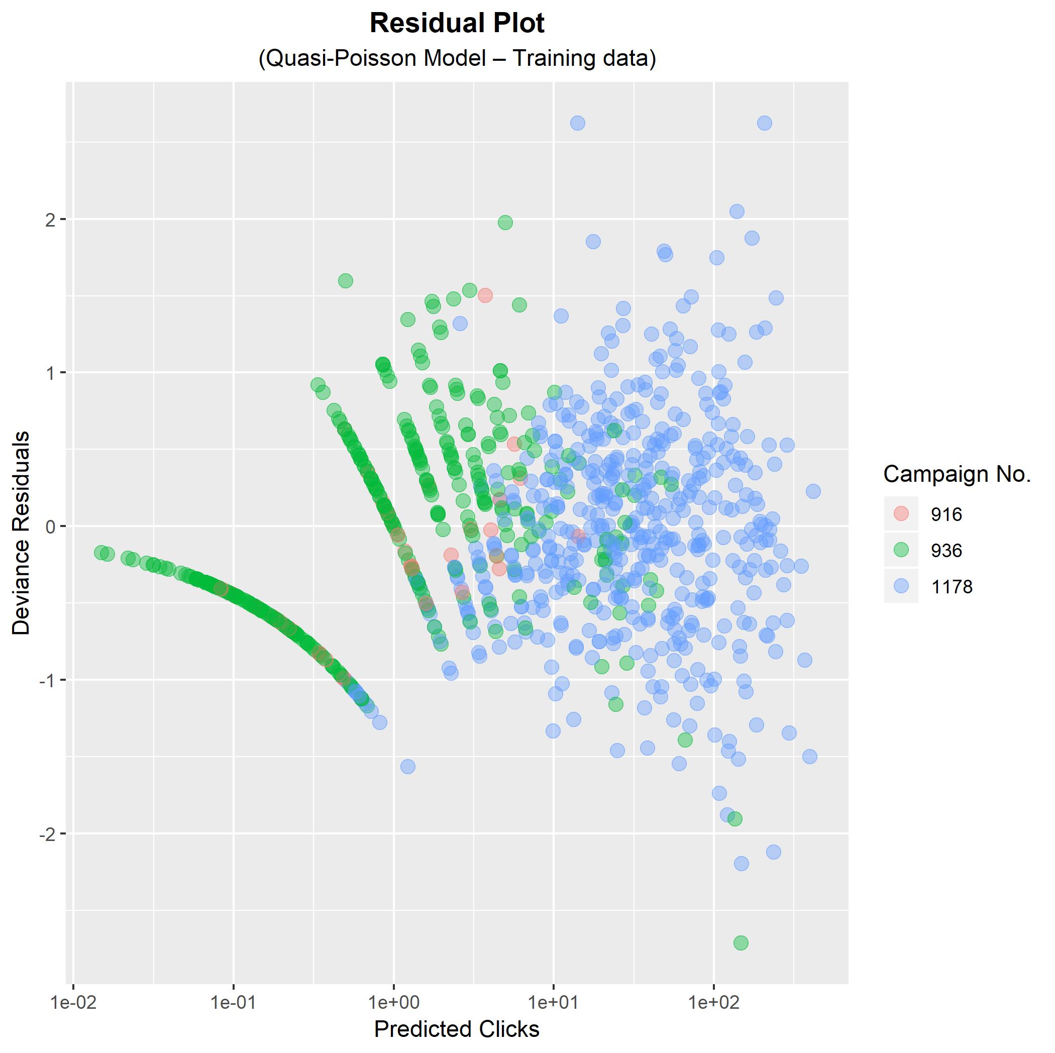
In the example here I have used a quasi-Poisson model, but the negative binomial model gives similar results. This model leads to a decent predictive model for Clicks, and implicitly for Clicks-per-Impression. It also gives a reasonable residual plot for the fitted model. It also gives an implicit estimate of the clicks-per-impressions for any input values of the other explanatory variables. The fitted model on the training data, excluding the coefficients for interest, yields:

                                  Estimate Std. Error t value Pr(>|t|)    
(Intercept)                      -7.896839   0.094512 -83.554  < 2e-16 ***
I(log(Spent + 0.01))              0.086426   0.004984  17.340  < 2e-16 ***
       ...
factor(xyz_campaign_id)936       -0.410562   0.079494  -5.165 2.99e-07 ***
factor(xyz_campaign_id)1178      -0.839471   0.079674 -10.536  < 2e-16 ***
factor(age)30-34:factor(gender)F -0.111433   0.015510  -7.185 1.45e-12 ***
factor(age)35-39:factor(gender)F  0.145936   0.016643   8.769  < 2e-16 ***
factor(age)40-44:factor(gender)F  0.272116   0.016361  16.632  < 2e-16 ***
factor(age)45-49:factor(gender)F  0.292668   0.014253  20.534  < 2e-16 ***
factor(age)30-34:factor(gender)M -0.415893   0.016504 -25.199  < 2e-16 ***
factor(age)35-39:factor(gender)M -0.243519   0.019479 -12.502  < 2e-16 ***
factor(age)40-44:factor(gender)M -0.082256   0.018197  -4.520 7.03e-06 ***

---
Signif. codes:  0 ‘***’ 0.001 ‘**’ 0.01 ‘*’ 0.05 ‘.’ 0.1 ‘ ’ 1

(Dispersion parameter for quasipoisson family taken to be 0.4400126)

    Null deviance: 2909.78  on 913  degrees of freedom
Residual deviance:  398.51  on 864  degrees of freedom

The ANOVA for the model is:

                           Df Deviance Resid. Df Resid. Dev
NULL                                         913    2909.78
I(log(Spent + 0.01))        1   199.72       912    2710.05
factor(interest)           39   435.64       873    2274.41
factor(xyz_campaign_id)     2   501.94       871    1772.47
factor(age):factor(gender)  7  1373.96       864     398.51

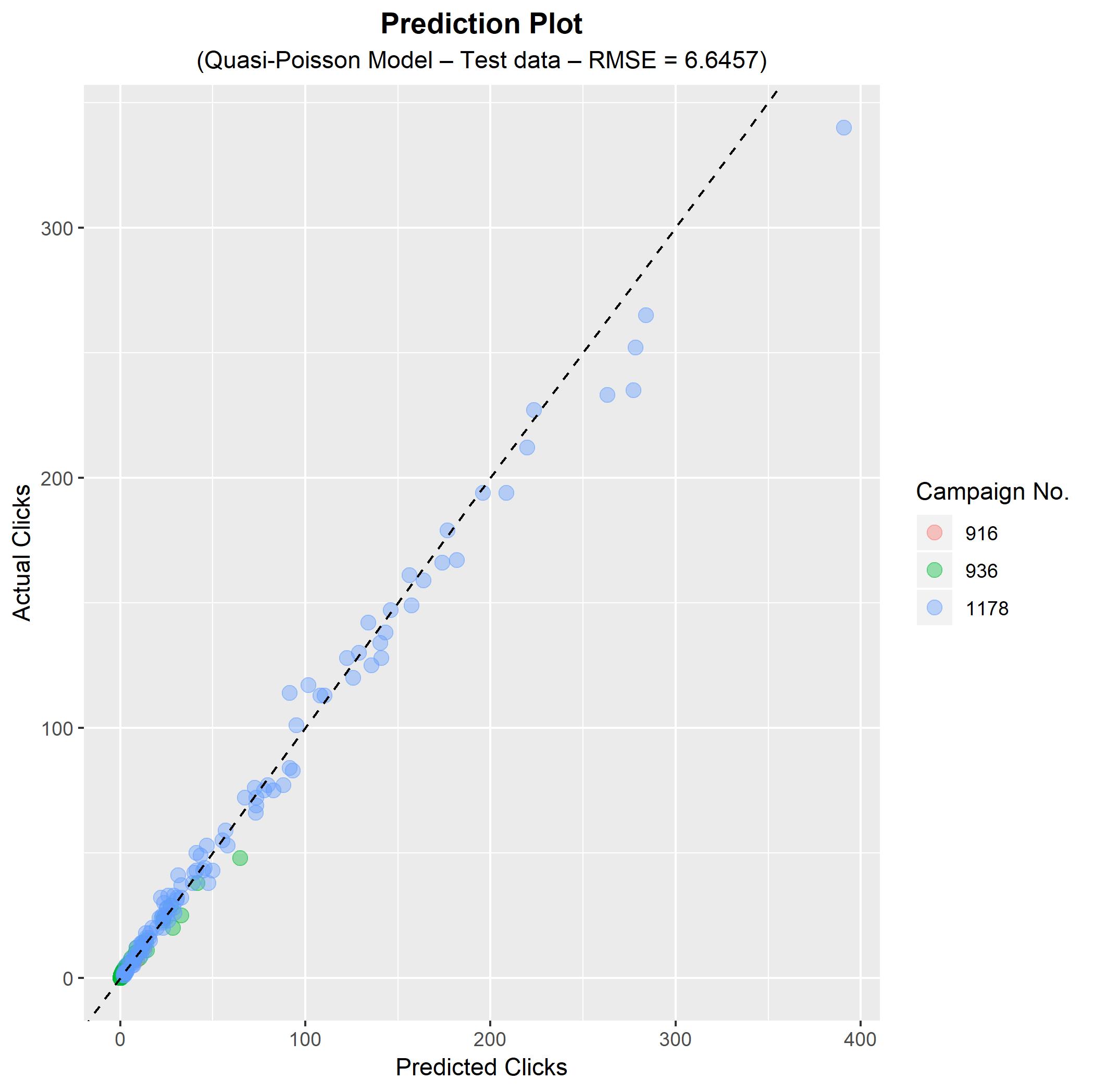
The predictions from applying the fitted model to the test data yield RMSE = 6.6457, and the prediction plots shows that there is some difficulty in predicting outcomes for ads with high numbers of predicted clicks. The residual and prediction plots are shown below. As can be seen from the plots and the summary output for the model, there is a substantial difference between the three campaigns in the data.

---

How does this help in understanding the clicks-per-impression? I noted above that this model form, which works with the raw count values, gives you an implicit predictive equation for the rate variable formed by the taking the ratio of Clicks on Impressions. To see why this is the case, we observe that (using the above coefficients) our fitted regression equation is:

$$\ln(\widehat{\text{Clicks}}) = \ln(\text{Impressions}) - 7.896839 + 0.086426 \ln(\text{Spent}) + \cdots .$$

Rearranging this equation yields:

$$\frac{\widehat{\text{Clicks}}}{\text{Impressions}} = \exp(- 7.896839) \times \text{Spent}^{0.086426} \times \cdots .$$

The left-hand-side of this equation functions as a rough estimator of the clicks-per-impression, and thus, your model allows you to make estimates of this rate measure. (There are a few technical issues with using this as an estimator. It is notable that non-linear functions of the predicted response are biased estimators of the corresponding non-linear function of the actual response, so the above equation gives a biased estimator of the clicks-per-impression. With non-linear transforms it is better to deal with the transformed response by looking at confidence intervals formed from the fitted model and then back-transforming these intervals. A detailed discussion of this issue is beyond the scope of this post, but the point here is that you can get an estimator of the rate measure from a model that operates on the raw count values.)

This shows you the method by which you can use a GLM for count values to obtain an implicit estimator of a rate measure formed as the ratio of two count values. The advantage of this method is that models designed to deal with count values often fit this data particularly well, and naturally take account of the heteroscedasticity that occurs with respect to the count variables. As noted, the present answer uses a different set of count variables than the ones you are interested in, but the method could be adapted to the rate measure of interest to you.

---

R code: Here is the R code used for the above plots and output:

######################### GET DATA #########################

#Load libraries
library(MASS);
library(ggplot2);

#Download the data
FILE <- 'http://rhokat.wdfiles.com/local--files/home%3Ahome/conversion_data.csv';
DATA <- read.csv(FILE, sep = ',')

#Split into training and testing data
#Replicates analysis in the question
#PROP is the proportion of data put in the training set
set.seed(100);
PROP       <- 0.8;
INDEX      <- sample(1:nrow(DATA), PROP*nrow(DATA));
DATA_TRAIN <- DATA[INDEX,  ];
DATA_TEST  <- DATA[-INDEX, ];

######################### FIT MODEL ########################

#Fit a quasi-Poisson model to the training data
MODEL_FORM <- as.formula(Clicks ~ offset(log(Impressions)) 
                                + I(log(Spent+0.01))
                                + factor(age):factor(gender) 
                                + factor(interest)
                                + factor(xyz_campaign_id));
MODEL      <- glm(MODEL_FORM, family = 'quasipoisson', data = DATA_TRAIN);

#Add fitted values and deviance residuals to data
DATA_TRAIN$Fitted   <- fitted(MODEL);
DATA_TRAIN$Residual <- residuals(MODEL, 'deviance');

#Generate the residual plot
RES_PLOT <- ggplot(data = DATA_TRAIN, 
                   aes(x = Fitted, y = Residual,
                       colour = factor(xyz_campaign_id))) +
            geom_point(alpha = 0.4, size = 3) +
            scale_x_log10() +
            scale_colour_discrete(name = 'Company No.') +
            theme(plot.title = element_text(hjust = 0.5, face = 'bold'),
                  plot.subtitle = element_text(hjust = 0.5)) +
            ggtitle('Residual Plot') +
            labs(subtitle = '(Quasi-Poisson Model – Training data)') +
            xlab('Predicted Clicks') + ylab('Deviance Residuals');
RES_PLOT;

#Generate ANOVA for model
anova(MODEL);

##################### MAKE PREDICTIONS #####################

#Apply the model to make predications on the test data
DATA_TEST$Clicks_Pred <- exp(predict(MODEL, newdata = DATA_TEST));
RMSE <- sqrt(mean((DATA_TEST$Clicks - DATA_TEST$Clicks_Pred)^2));

#Generate the prediction plot
SUBTITLE <- paste0('(Quasi-Poisson Model – Test data – RMSE = ', 
round(RMSE,4), ')');
PRED_PLOT <- ggplot(data = DATA_TEST, 
                    aes(x = Clicks_Pred, y = Clicks, 
                        colour = factor(xyz_campaign_id))) +
            geom_point(alpha = 0.4, size = 3) +
            geom_abline(slope = 1, linetype = 'dashed') +
            scale_colour_discrete(name = 'Company No.') +
            scale_x_continuous() +
            scale_y_continuous() +
            theme(plot.title = element_text(hjust = 0.5, face = 'bold'),
                  plot.subtitle = element_text(hjust = 0.5)) +
            ggtitle('Prediction Plot') +
            labs(subtitle = SUBTITLE) +
            xlab('Predicted Clicks') + ylab('Actual Clicks');
PRED_PLOT;

---

$^\dagger$ Some preliminary exploratory analysis shows that the variable fb_campaign_id is nested within xyz_campaign_id and this is too detailed, since it perfectly predicts several values in combination with the other factors. Using this variable would overfit the model so we omit it.

$^{\dagger \dagger}$ If I were doing a proper analysis I would try to avoid variable-padding for a log variable, since this has the side-effect of making your analysis depend on the arbitrary padding value. In this case the output is reasonably robust to this value, and I am only fitting an example model.

Answer 2

I downloaded the data from your link and attempted to recreate your problem.

The first thing I did is to convert the campaign id to a factor:

data$xyz_campaign_id <- as.factor(data$xyz_campaign_id)

Next I ran a linear model to predict Total Conversion using the variables you specified in your example.

simple_linear <- lm(Total_Conversion ~ gender + interest + Clicks + Spent + Impressions + xyz_campaign_id, data = data)

I then checked the model output by running summary(simple_linear), and got a high adjusted R-squared value of 0.73 showing that this model explains approximately 73% of the variation in the data.

To improve the model I explored the effect that interactions could have on model fit.

See this wikipedia article for more information on interactions.

Example code on constructing various models with varying interaction terms:

simple_linear.1int <- lm(Total_Conversion ~ gender + interest + Clicks * Spent + Impressions + xyz_campaign_id, data = data) 

simple_linear.2int <- lm(Total_Conversion ~ gender + interest + Clicks * Spent * Impressions + xyz_campaign_id, data = data) 

simple_linear.3int <- lm(Total_Conversion ~ gender + interest * Clicks * Spent * Impressions + xyz_campaign_id, data = data) 

simple_linear.4int <- lm(Total_Conversion ~ gender * interest * Clicks * Spent * Impressions + xyz_campaign_id, data = data) 

We can now compare these models using the Akaike Information Criterion which gives us an estimate of the quality of a statistical model (the lower the value the better the model when comparing it against others).

# AIC criterion calculation for every model

AIC(simple_linear)
AIC(simple_linear.1int)
AIC(simple_linear.2int)
AIC(simple_linear.3int)
AIC(simple_linear.4int)

When now running summary() again for every model, the one with 4 interaction terms now has the highest R-squared value and the lowest AIC value, and therefore represents an improvement over the simple linear model.

Answer 3

Good p but low R2

This is not a strange situation since you have a lot of data points. You are dealing with a sort of law of large numbers (decreasing probability for small deviation of the mean for large number of data).

For larger number of data small deviations of the trend line (R2 is deviation of trend line divided by deviation of the data) become less probable. See the images below for example.

set.seed(1)
layout(matrix(1:3,1))

for (i in 1:3) {
  n <- c(5,10,100)[i]
  p <- 0
  r <- 0
  pmod <- 0
  for (t in 1:5000) {
    y <- rnorm(n,0,1)
    x <- seq(0,10,length.out=n)
    mod <- lm(y~x)
    anv <- anova(mod)
    if (abs(anv$`Pr(>F)`[1]-0.01) < abs(p-0.01)) {
  pmod <- mod
  p <- anv$`Pr(>F)`[1]
      r <- var(predict(mod)/var(y))
    }
  }
  plot(x,y,
       xlim=c(0,10),ylim=c(-2.5,2.5))
  lines(x,predict(mod))
  Lines <- list(bquote(paste("n = ",.(n))),bquote(paste("p = ",.(round(p,5)))),bquote(paste("R"^2," = ",.(round(r,3)))))
  mtext(do.call(expression, Lines),side=3,line=2:0, cex=0.7)
}

---

Improvement of model

Your data is basically data of success and failure. For each click/impression you may or may not get a click/conversion. This can be modeled as binomial distributed data (you model the probability to get a success as a function of the variables like campaign gender and interest).

Then it is better to use a generalized linear model instead of an ordinary linear regression (it allows a link function but most important of all it allows to model probability of the erro differently, as binary data instead of gaussian distributed data).

Below is an example how to put it in code:

data$y <- cbind(data$Total_Conversion,data$Impressions-data$Total_Conversion)

data[1,]

mod <- glm(y ~ as.factor(xyz_campaign_id) + 
               as.factor(age) + 
               as.factor(gender) + 
               as.factor(interest) , family = binomial(), data=data)

summary(mod)

> summary(mod)

Call:
glm(formula = y ~ as.factor(xyz_campaign_id) + as.factor(age) + 
    as.factor(gender) + as.factor(interest), family = binomial(), 
    data = data)

Deviance Residuals: 
    Min       1Q   Median       3Q      Max  
-4.8862  -0.4765   0.3319   1.0702   5.7332  

Coefficients:
                               Estimate Std. Error z value Pr(>|z|)    
(Intercept)                    -8.35436    0.21102 -39.590  < 2e-16 ***
as.factor(xyz_campaign_id)936  -0.31878    0.14020  -2.274  0.02299 *  
as.factor(xyz_campaign_id)1178 -2.33740    0.13557 -17.241  < 2e-16 ***
as.factor(age)35-39            -0.31129    0.04921  -6.326 2.52e-10 ***
as.factor(age)40-44            -0.47718    0.05351  -8.917  < 2e-16 ***
as.factor(age)45-49            -0.74920    0.04900 -15.288  < 2e-16 ***
as.factor(gender)M              0.24957    0.03892   6.413 1.42e-10 ***
as.factor(interest)7           -0.16451    0.20515  -0.802  0.42260    
as.factor(interest)10          -0.41185    0.17030  -2.418  0.01559 *  
as.factor(interest)15          -0.38375    0.17425  -2.202  0.02764 *  
as.factor(interest)16          -0.84690    0.16783  -5.046 4.51e-07 ***
as.factor(interest)18          -0.77352    0.19269  -4.014 5.96e-05 ***
as.factor(interest)19          -0.25322    0.18817  -1.346  0.17840    
as.factor(interest)20          -0.23804    0.18131  -1.313  0.18923    
as.factor(interest)21           0.14531    0.19889   0.731  0.46502    
as.factor(interest)22          -0.65382    0.21273  -3.073  0.00212 ** 
as.factor(interest)23          -0.19944    0.24408  -0.817  0.41386    
as.factor(interest)24          -0.20747    0.22375  -0.927  0.35378    
as.factor(interest)25          -0.33910    0.19485  -1.740  0.08181 .  
as.factor(interest)26          -0.49123    0.19806  -2.480  0.01313 *  
as.factor(interest)27          -0.45564    0.17210  -2.648  0.00811 ** 
as.factor(interest)28          -0.57311    0.17881  -3.205  0.00135 ** 
as.factor(interest)29          -0.33412    0.16888  -1.978  0.04788 *  
as.factor(interest)30          -0.20310    0.21990  -0.924  0.35569    
as.factor(interest)31           0.37680    0.23585   1.598  0.11013    
as.factor(interest)32          -0.49900    0.19566  -2.550  0.01076 *  
as.factor(interest)36           0.20341    0.24657   0.825  0.40940    
as.factor(interest)63          -0.48914    0.18826  -2.598  0.00937 ** 
as.factor(interest)64          -0.34273    0.19310  -1.775  0.07591 .  
as.factor(interest)65          -0.27561    0.23590  -1.168  0.24269    
as.factor(interest)66          -0.47645    0.31082  -1.533  0.12531    
as.factor(interest)100          0.36159    0.22934   1.577  0.11488    
as.factor(interest)101          0.38336    0.19991   1.918  0.05515 .  
as.factor(interest)102         -0.30425    0.31133  -0.977  0.32843    
as.factor(interest)103         -0.49026    0.27085  -1.810  0.07029 .  
as.factor(interest)104          0.67505    0.22212   3.039  0.00237 ** 
as.factor(interest)105         -0.35516    0.23820  -1.491  0.13596    
as.factor(interest)106         -0.22747    0.27586  -0.825  0.40961    
as.factor(interest)107         -0.19347    0.20202  -0.958  0.33823    
as.factor(interest)108         -0.18805    0.23327  -0.806  0.42015    
as.factor(interest)109         -0.17986    0.22852  -0.787  0.43126    
as.factor(interest)110         -0.13102    0.23032  -0.569  0.56945    
as.factor(interest)111          0.05861    0.24320   0.241  0.80955    
as.factor(interest)112          0.25045    0.21119   1.186  0.23565    
as.factor(interest)113         -0.16450    0.25586  -0.643  0.52027    
as.factor(interest)114         -0.15016    0.33078  -0.454  0.64986    
---
Signif. codes:  0 ‘***’ 0.001 ‘**’ 0.01 ‘*’ 0.05 ‘.’ 0.1 ‘ ’ 1

(Dispersion parameter for binomial family taken to be 1)

    Null deviance: 3212.1  on 1142  degrees of freedom
Residual deviance: 1619.0  on 1097  degrees of freedom
AIC: 4579.6

Number of Fisher Scoring iterations: 6

The actual implementation in the GLM function is not so important for this particular case. For low probabilities of success and high number of trials the binomial distribution is almost the same as the Poisson distribution, and also the link functions are similar in the tail, e.g. $log(p) \approx log(\frac{p}{1-p}) $

---

How good is the model?

I would not use $R^2$ for this type of data (instead use $\chi^2$ to measure goodness of fit). This is because you naturally have a variation in the data because it is Poisson/Binomial distributed or according to some other distribution of counts that is a sum of Bernoulli trials.

For instance, imagine you have to model coins that have probability for heads and tails between 0.49 and 0.51. Then your model may very accurately model this small variation (between coins) in the probability, but the data may have a large variation (within repeated flips of a single coin). E.g. if you flip a coin 10 times then it will have a mean close to 5 times heads, but the variance will be 2.5 and you will have a large $R^2$ but your model can not be much better (the data varies with 2.5 but your model only differs between 0.49 and 0.51 for the probability of heads and tails).

Something similar occurs when you will model the probability of an impression turning into a click. The model will be over-fitted (even though the $R^2$ is only around 0.25)

See the images below (generated with the code below)

• left a plot of predicted clicks vs observed clicks
• right a plot of modeled data (average of ten repetitions) using binomial distribution with the predicted value for the probability of v click and the observed number of impressions as the number of trials.

Note that the observations are more close to the predictions than the modeled data. This indicates over-fitting (or under-dispersion, making us model the data with too large variance).

The imaged below show the results of a Monte Carlo simulation (10 000 times) to estimate the distribution for $\chi^2$ and $R^2$. The values for the model are:

> # compute chi-sq
> sum(((npred-data$Clicks)^2/npred))
[1] 586.4344
> # compute R^2
> var(predict(mod, type='response')) / var(data$Clicks/data$Impressions)
[1] 0.275814

The low chi-square value (and also the relatively high $R^2$) indicate that the fit is too good to be true.

It would be much more plausible to observe $R^2$ around 0.10 and it should not be expected that a model with a higher value is truly a better model. To expect a low $R^2$ is simply due to the variability of the measurements, that are comparable to the variability in the example with the coin flips.

Small note: when you model the conversions/impressions then you do get a lower $R^2$ and higher $\chi^2$ than expected.

# create data column for binomial model
data$y <- cbind(data$Clicks,data$Impressions-data$Clicks)

# model
mod <- glm(y ~ as.factor(xyz_campaign_id) + 
               (as.factor(age) + 
               as.factor(gender) + 
               as.factor(interest)) , family = binomial(link='logit'), data=data)

# print results
summary(mod)


# compare deviation of predictions with monte carlo
set.seed(1)
layout(matrix(1:2,1))

# prediction of counts
npred <- predict(mod, type='response')*data$Impressions

# plot vs observations
plot(npred[which(as.factor(data$xyz_campaign_id)!=1)],data$Clicks[which(as.factor(data$xyz_campaign_id)!=1)],
     pch=21,col=rgb(0,0,0,0.1),bg=rgb(0,0,0,0.1),cex=0.7,log="",
     xlim = c(0,365),ylim=c(0,365),
     xlab = "n predicted", ylab = "n observed")

# plot vs modelled data
plot(-100,-100,
     pch=21,col=rgb(0,0,0,0.01),bg=rgb(0,0,0,0.01),cex=0.7,log="",
     xlim=c(0,365),ylim=c(0,365),
     xlab = "n predicted", ylab = "y modeled")
for (i in 1:10) {
  test <- rbinom(length(npred),data$Impressions,predict(mod,type='response'))
  points(npred,test,
       pch=21,col=rgb(0,0,0,0.01),bg=rgb(0,0,0,0.01),cex=0.7)
}

# compute chi-sq
sum(((npred-data$Clicks)^2/npred))
# compute R^2
var(predict(mod, type='response')) / var(data$Clicks/data$Impressions)


# compare with monte carlo simulation
v_chi <- rep(0,10000)
v_p <- rep(0,10000)
for (i in 1:10000) {
  test <- rbinom(length(npred),data$Impressions,predict(mod,type='response'))
  v_chi[i] <- sum(((npred-test)^2/npred))
  v_p[i] <- var(predict(mod, type='response'))/var(test/data$Impressions)
}
hist(v_chi, xlab=expression(chi^2),main=expression(paste("Histogram of ",chi^2," for modeled data")))
hist(v_p, xlab=expression(R^2),main=expression(paste("Histogram of ",R^2," for modeled data")))

Answer 4

Consider what look like CR outliers to address in different possible ways (cross-validation, downweight/transform/delete). Prior comments on interactions would seem helpful, and squared terms might be worth exploring.