Assume first the the parameters $\boldsymbol\mu$ and $\boldsymbol\Sigma$ are known. Just as $\frac{x-\mu}\sigma$ is standard normal and $\frac{(x-\mu)^2}{\sigma^2}$ chi-square with 1 degree of freedom in the univariate case, the quadratic form
$(\mathbf{x}-\boldsymbol\mu)^T\boldsymbol\Sigma^{-1}(\mathbf{x}-\boldsymbol\mu)$ is chi-square with $p$ degrees of freedom when $\mathbf{x}$ is multivariate normal. Hence, this pivot
$$
(\mathbf{x}-\boldsymbol\mu)^T\boldsymbol\Sigma^{-1}(\mathbf{x}-\boldsymbol\mu)\le \chi_{p,\alpha}^2 \tag{1}
$$
with probability $(1-\alpha)$. A probability region for $\mathbf{x}$ is found by inverting (1) with respect to $\mathbf{x}$. For points at the boundary of this set, ${\mathbf{L}^{-1}}(\mathbf{x}-\boldsymbol{\mu})$ lies on a circle with radius $\sqrt{\chi^2_{p,\alpha}}$ where $\mathbf L$ is the cholesky factor of $\boldsymbol\Sigma$ (or some other square root) such that
$$
\mathbf{L}^{-1}(\mathbf{x}-\boldsymbol{\mu})=\sqrt{\chi^2_{p,\alpha}}
\left[
\begin{matrix}
\cos(\theta)\\
\sin(\theta)
\end{matrix}
\right].
$$
Hence, the boundary of the set (an ellipse) is described by the parametric curve
$$
\mathbf{x}(\theta)=
\boldsymbol{\mu} + \sqrt{\chi^2_{p,\alpha}}\mathbf{L}
\left[
\begin{matrix}
\cos(\theta)\\
\sin(\theta)
\end{matrix}
\right],
$$
for $0<\theta <2\pi$.
If the parameters are unknown and we we use $\bar{\mathbf{x}}$ to estimate $\boldsymbol\mu$, $\mathbf{x}-\bar{\mathbf{x}} \sim N_p(0,(1+1/n))\boldsymbol{\Sigma})$. Hence, $(1+1/n)^{-1}(\mathbf{x}-\bar{\mathbf{x}})^T\boldsymbol\Sigma^{-1}(\mathbf{x}-\bar{\mathbf{x}})$ is chi-square with $p$ degrees of freedom. Substituting $\boldsymbol\Sigma$ by its estimate $\hat{\boldsymbol\Sigma}=\frac1{n-1}\mathbf{X}^T \mathbf{X}$ the resulting pivot is instead Hotelling $T$-squared distributed with $p$ and $n-p$ degrees of freedom (analogous to the $F_{1,n-1}$ distributed squared $t$-statistic in the univariate case) such that
$$
\Big(1+\frac1n\Big)^{-1}(\mathbf{x}-\bar{\mathbf{x}})^T\hat{\boldsymbol\Sigma}^{-1}(\mathbf{x}-\bar{\mathbf{x}})
\le T^2_{p,n-p,\alpha} \tag{2}
$$
with probability $(1-\alpha)$. Because the Hotelling $T$-squared is just a rescaled $F$-distribution, the above quantile equals $\frac{p(n-1)}{n-p}F_{p,n-p,\alpha}$.
Inverting (2) with respect to $\mathbf{x}$ leads to a prediction region with boundary described by the parametric curve
$$
\mathbf{x}(\theta)=
\bar{\mathbf x} + \sqrt{\Big(1+\frac1n\Big)\frac{p(n-1)}{n-p}F_{p,n-p,\alpha}}\hat{\mathbf{L}}
\left[
\begin{matrix}
\cos(\theta)\\
\sin(\theta)
\end{matrix}
\right]
$$
where $\hat{\mathbf L}$ is the cholesky factor of the sample variance matrix $\hat{\boldsymbol\Sigma}$.
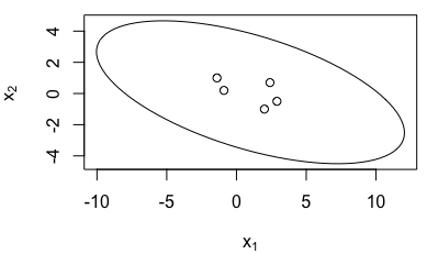
Code computing this for the data in the original question:
pred.int.mvnorm <- function(x, alpha=.05) {
  p <- ncol(x)
  n <- nrow(x)
  Sigmahat <- var(x)
  xbar <- apply(x,2,mean)
  xbar
  theta <- seq(0, 2*pi, length=100)
  polygon <- xbar +
    sqrt(p*(n-1)/(n-p)*(1 + 1/n)*qf(alpha, p, n - p, lower.tail = FALSE))*
    t(chol(Sigmahat)) %*%
    rbind(cos(theta), sin(theta))
  t(polygon)
}
x <- matrix(c(-0.9,2.4,-1.4,2.9,2.0,0.2,0.7,1.0,-0.5,-1.0),ncol=2)
plot(pred.int.mvnorm(x), type="l",xlab=expression(x[1]),ylab=expression(x[2]))
points(x)

More code testing the coverage
library(mvtnorm)
library(sp)
hits <- 0
for (i in 1:1e+5) {
  x <- rmvnorm(6, sigma = diag(2))
  pred.int <- pred.int.mvnorm(x[-1,])
  x <- x[1,]
  if (point.in.polygon(x[1], x[2], pred.int[,1], pred.int[,2])==1)
    hits <- hits + 1
}
hits
[1] 94955

