From 43 years of monthly stream flow data, I want to get 11 years ARIMA future forecast using Minitab 15 statistical Software.
The difficulty is the procedure to be followed, interpretation of model outputs (Final Estimates of Parameters and Modified Box-Pierce (Ljung-Box) Chi-Square statistics) and other best fit model selection criteria like AIC, BIC etc. Any one who can help me is appreciated. The raw data:
2.76
2.11
1.7
1.25
1.25
2.14
19.27
42.97
21.54
6.95
3.68
2.87
2.18
1.83
1.57
1.38
1.08
2.17
24.52
33.48
24.86
9.86
7.55
6.05
2.61
1.71
1.56
1.01
1.21
2.13
18.08
31.41
22.5
8.18
4.3
2.97
2.2
1.54
1.46
1.35
1.8
2.84
18.33
34.43
20.46
6.25
7.72
4.29
2.43
1.49
1.13
1.2
1.43
2.94
42.58
51.32
30.71
13
6.12
3.95
2.68
2.06
2.01
1.71
1.26
2.37
11.52
26.97
14.76
10.5
7.43
4.33
2.16
1.62
1.55
1.16
1.33
2.16
16.43
25.17
17.43
4.81
3.39
2.29
1.73
1.38
1.46
1.15
1.06
3.11
24.04
35.75
23.49
9.82
4.44
3.13
2.54
1.77
1.7
1.35
1.42
4.65
32.49
27.43
19.49
5.02
4.86
5.02
2.35
1.76
1.8
1.36
1.39
3.04
31.74
51.66
27.06
6.78
4.06
3.21
2.03
1.71
1.66
1.45
2.4
5.38
22.52
38.41
21.69
7.58
3.69
2.64
2.02
1.55
1.36
1.15
1.22
3.5
18.3
41.48
21.6
6.71
5.08
2.85
2.19
1.41
1.28
1.07
1.11
2.73
10.74
21.15
14.17
4.18
2.87
1.75
1.34
0.98
0.89
0.79
1.12
2.47
13.34
46.49
17.1
7.07
3.34
2.32
1.84
1.3
1.21
0.96
2.23
3.18
25.22
35.36
27.7
8.21
3.94
2.7
2.17
2.11
1.61
1.23
1.26
3.9
49.69
96.27
67.47
17.04
6.28
6.01
3.48
3.36
3.06
2.5
3.52
14.98
28.34
44.81
24.12
7.49
5.12
3.13
2.29
1.55
1.47
1.09
1
2.88
19.7
24.31
15.24
14.28
4.27
2.53
2.42
1.63
1.43
1.46
1.63
8.79
33.17
32.96
26.45
8.96
4.56
3.43
2.49
1.7
1.48
1.17
1.53
3.3
14.07
29.24
19.26
7.79
3.14
2.29
1.65
1.27
1.16
1.15
1.16
7.56
34.35
34.35
12.84
6.6
2.8
2.06
1.73
1.39
1.43
0.96
1.81
4.73
42.59
35.78
26.99
7.51
2.64
1.97
1.79
1.52
1.73
1.42
1.67
6.25
26.93
32.81
21.82
7.99
2.6
1.99
1.54
1.11
1.12
0.85
0.89
3.56
5.86
39.91
14.07
6.66
2.89
1.91
1.36
0.89
0.89
0.78
0.9
10.72
22.42
21.67
17.46
4.62
2.55
2.16
1.37
0.93
0.84
0.75
1.01
3.84
15.71
32.72
16.24
5.93
3.36
2.1
1.49
0.94
0.85
0.65
0.55
3.57
14.13
15.95
15.58
7.45
2.85
2.19
1.57
1.21
1.71
0.89
2.33
9.44
15.77
19.92
12.85
6.6
3.56
2.41
1.99
1.3
1.17
0.7
1.02
6.34
40.25
35.71
26.34
15.6
5.03
3.17
2.41
1.55
1.47
1.19
1.41
7.93
27.54
32.99
16.63
6.4
3.09
1.87
1.43
1.46
1.35
1.06
1.13
2.08
18.02
56.17
21.99
5.82
2.95
2.09
1.62
1.11
1.02
1.28
1.35
4.47
31.81
55.78
26.49
6.13
4.73
3.49
2.55
1.68
1.55
1.49
1.46
3.17
16.67
40.25
20.07
14.23
7.77
4.15
3.6
2.33
1.8
1.74
2.24
7.87
32.87
25.45
24.42
11.17
5.4
3.32
2.32
1.62
1.48
1.22
1.46
6.09
17.88
23.93
21.77
5.89
4.06
2.85
1.9
1.33
1.32
1.17
1.65
5.15
17.28
29.62
21.1
5.25
3.04
2.29
1.71
1.09
1.21
1.55
3.31
14.33
34.6
42.93
24.74
9.36
4.67
3.3
2.47
1.7
1.63
1.27
2.76
8.08
20.12
28.48
14.6
11.18
6.93
3.42
2.33
1.5
1.33
1.09
2.52
7.16
23.86
34.65
25.07
19.58
6.41
4.27
3.06
1.95
1.62
1.35
2.24
10.19
38.02
33.4
20.03
19.02
5.96
4.27
2.61
1.72
1.52
1.88
1.85
5.4
18.6
53.81
19.31
23.97
8.04
3.92
2.6
1.92
1.79
1.4
1.99
11.96
37.47
54.03
17.56
7.41
4.1
3.06
2.38
1.67
1.64
1.29
1.21
5.55
19.57
32.44
15.63
6.24
3.45
2.11

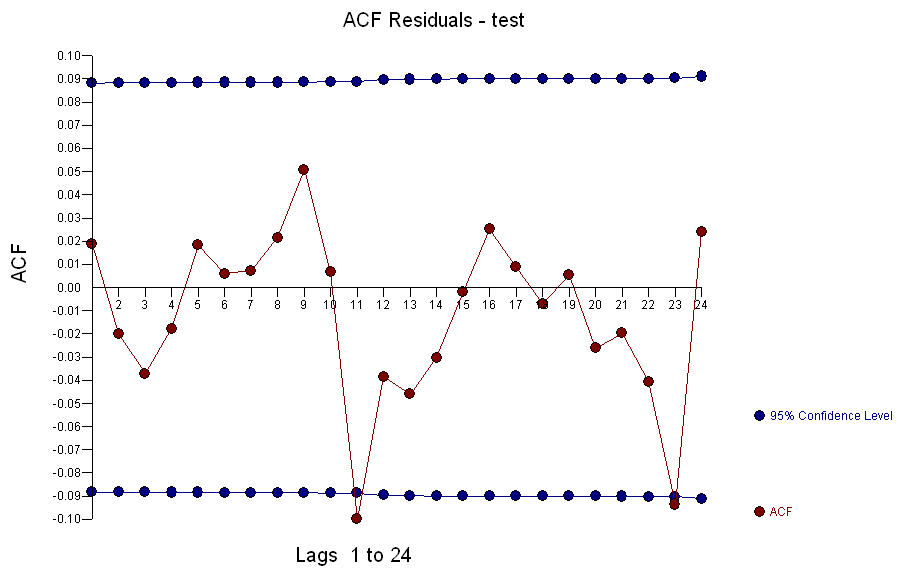
 . The time series is rich with ARIMA structure and Gaussian Violations which fortunately can be rectified. The underlying model is a (1,0,0)(1,1,0) with a large number of Pulse/One time anomnalies and a significant change point in the error variance (increase) at
  period 335. THe basic methodology is outlined in
  and an error process ACF of
  suggesting an adequate model. The forecast for the next 11 years is
  and the Actual-Fit-Forecast graph is
  . THe problem you are having trying to use minitab ( and other time series software ) is that the time series is more complicated than what their solution allows for. It would be interesting to compare the minitab model with the AUTOBOX model ( shown partially )