Introducing random slopes in nested model improves model fit but residuals variances become unequal

Question

I have measured boldness scores (continuous variable) across time (trials) for individuals (ID) within colonies (colony). The data is coded such that individuals 1-30 belong to one colony, 31-60 to the next colony and so on. I have 13 such colonies consisting of ~ 30 individuals each. Since the assumptions of normality of residuals was not met in a linear mixed effects model, I boxcox transformed the response variable (boldness score) and ran the model with this transformed response variable, trial as fixed effects and individuals nested within colonies (1|ID)+(1|colony) as random effects. The qq plot and residual plots below shows that the residuals are approximately normally distributes (though with a slight skew of $-0.0009$).

QQplot:

Residual Plot:

Now I want to see how boldness scores of colonies change over trials. So the model was lmer(Boldness~Trial+(1|ID)+(Trial|colony),data=mydata). This model seems to be a better fit than the model with random intercepts alone, as evident from significant deviance value. However, the residuals of this model is more skewed than the previous model ($0.04$) as evident from the qqplot:

QQplot with random slopes for colonies:

Residuals plot with random slopes for colonies:

As it is evident from the residuals plot, the residuals seem to have uneuqal variances. The question is if I should accept the random slope model as it explains greater variance than the intercept only model, or should I reject the random slope model as its model assumptions seems not to be met.

Answer 1

In your model, it appears that ID is nested in colony, in which case a cleaner way of writing your simpler model would be:

lmer(Boldness~Trial+(1|colony/ID),data=mydata).

Then, your more complicated model would be written like this:

lmer(Boldness~Trial+(1 + Trial|colony/ID),data=mydata).

In your question, you don't explicitly mention what your original inferential and/or predictive goals are for these data.

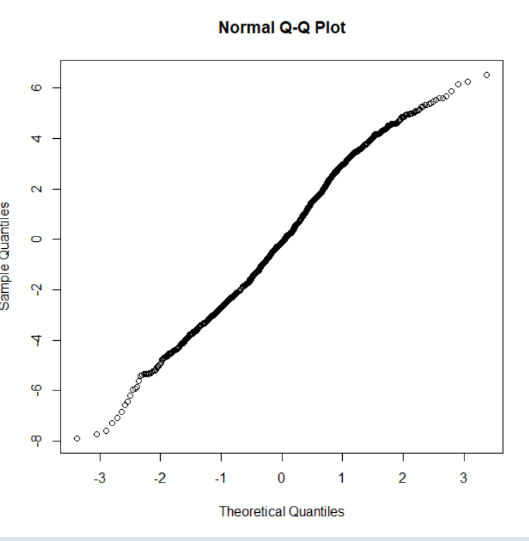
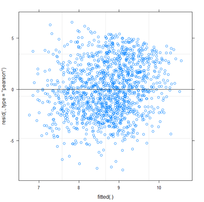
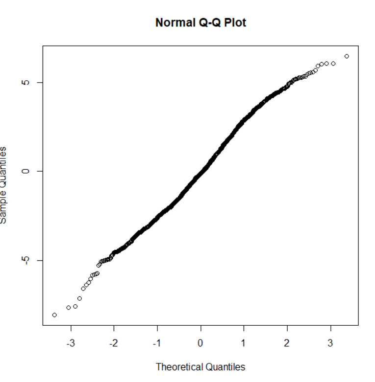
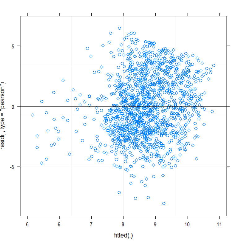
If you are originally interested in estimating the effect of Trial on (untransformed) Boldness for a typical individual within a typical colony, one possibility would be to fit your lmer model (whichever is more appropriate between the two listed above, based on AIC or BIC, for instance) to the untransformed Boldness and then use bootstrap to conduct inference on the effect of interest, as explained here: https://datascienceplus.com/introduction-to-bootstrap-with-applications-to-mixed-effect-models/. Using bootstrap would address the lack of normality of the residuals from the model based on the untransformed response, though of course you would still want no systematic features to be present in the plot of model residuals vs. fitted values (e.g., tendency of residuals to increase/decrease with the fitted values). If such systematic features are present, then you can use a Box-Cox transformation of the Boldness, fit your lmer model to the transformed Boldness and, if the model residuals do not look normally distributed (but no longer show systematic features when plotted against the fitted values), use bootstrap for conducting inferences.

Actually, if your model of the untransformed Boldness showed that its residuals increase (or decrease) as a function of the fitted model, you could explicitly model that increasing/decreasing variability of the model errors (rather than transforming Boldness to make it go away). Unfortunately, from what I know, lmer does not support this option, though lme does (lme comes from the nlme package).

Coming back to your question, I wanted to suggest that you give the DHARMa package a try to get more insights into the behaviour of the residuals for your models: https://cran.r-project.org/web/packages/DHARMa/vignettes/DHARMa.html.

Also, have a look at the AIC or BIC values for your two models, as well as the marginal and conditional R-squared values (which you can compute as explained at https://ecologyforacrowdedplanet.wordpress.com/2013/08/27/r-squared-in-mixed-models-the-easy-way/), as you need to better understand their relative performance prior to making a choice based on their model diagnostic performance.

In terms of which model to choose between your two models, remember that minor violations of the model assumptions are generally OK in practice. It's major violations that we should be concerned with as they can really invalidate model-based inferences and predictions.

If the AIC/BIC conparison and R-squared comparison of your two models reveal a gulf of difference between the two models (in favour of the more complex model, say) and the violations of the model assumptions you see in the diagnostic plots are minor, then you can feel justified in picking the more complex model and note that it comes with minor assumption violations, which won't be expected to have much impact on the validity of the model-based inferences and predictions.

If the AIC/BIC comparison and R-squared comparison of your two models reveal the models are 'close' in performance (e.g., AIC/BIC values are within 2 or 3 points of each other, marginal and conditional R-squared values are really close), then you'll probably want to pick the simpler model as it will be easier to interpret and then note to what extent it meets the underlying model assumptions.