This type of situation can be handled by a standard F-test for nested models. Since you want to test both of the parameters against a null model with fixed parameters, your hypotheses are:
$$H_0: \boldsymbol{\beta} = \begin{bmatrix} 0 \\ 1 \end{bmatrix} \quad \quad \quad H_A: \boldsymbol{\beta} \neq \begin{bmatrix} 0 \\ 1 \end{bmatrix} .$$
The F-test involves fitting both models and comparing their residual sum-of-squares, which are:
$$SSE_0 = \sum_{i=1}^n (y_i-x_i)^2 \quad \quad \quad SSE_A = \sum_{i=1}^n (y_i - \hat{\beta}_0 - \hat{\beta}_1 x_i)^2$$
The test statistic is:
$$F \equiv F(\mathbf{y}, \mathbf{x}) = \frac{n-2}{2} \cdot \frac{SSE_0 - SSE_A}{SSE_A}.$$
The corresponding p-value is:
$$p \equiv p(\mathbf{y}, \mathbf{x}) = \int \limits_{F(\mathbf{y}, \mathbf{x}) }^\infty \text{F-Dist}(r | 2, n-2) \ dr.$$
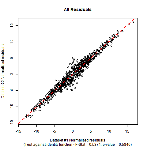
Implementation in R: Suppose your data is in a data-frame called DATA with variables called y and x. The F-test can be performed manually with the following code. In the simulated mock data I have used, you can see that the estimated coefficients are close to the ones in the null hypothesis, and the p-value of the test shows no significant evidence to falsify the null hypothesis that the true regression function is the identity function.
#Generate mock data (you can substitute your data if you prefer)
set.seed(12345);
n    <- 1000;
x    <- rnorm(n, mean = 0, sd = 5);
e    <- rnorm(n, mean = 0, sd = 2/sqrt(1+abs(x)));
y    <- x + e;
DATA <- data.frame(y = y, x = x);

#Fit initial regression model
MODEL <- lm(y ~ x, data = DATA);

#Calculate test statistic
SSE0   <- sum((DATA$y-DATA$x)^2);
SSEA   <- sum(MODEL$residuals^2);
F_STAT <- ((n-2)/2)*((SSE0 - SSEA)/SSEA);
P_VAL  <- pf(q = F_STAT, df1 = 2, df2 = n-2, lower.tail = FALSE);

#Plot the data and show test outcome
plot(DATA$x, DATA$y,
     main = 'All Residuals',
     sub  = paste0('(Test against identity function - F-Stat = ',
            sprintf("%.4f", F_STAT), ', p-value = ', sprintf("%.4f", P_VAL), ')'),
     xlab = 'Dataset #1 Normalized residuals',
     ylab = 'Dataset #2 Normalized residuals');
abline(lm(y ~ x, DATA), col = 'red', lty = 2, lwd = 2);
The summary output and plot for this data look like this:
summary(MODEL);

Call:
lm(formula = y ~ x, data = DATA)

Residuals:
    Min      1Q  Median      3Q     Max
-4.8276 -0.6742  0.0043  0.6703  5.1462

Coefficients:
            Estimate Std. Error t value Pr(>|t|)
(Intercept) -0.02784    0.03552  -0.784    0.433
x            1.00507    0.00711 141.370   <2e-16 ***
---
Signif. codes:  0 ‘***’ 0.001 ‘**’ 0.01 ‘*’ 0.05 ‘.’ 0.1 ‘ ’ 1

Residual standard error: 1.122 on 998 degrees of freedom
Multiple R-squared:  0.9524,    Adjusted R-squared:  0.9524
F-statistic: 1.999e+04 on 1 and 998 DF,  p-value: < 2.2e-16

F_STAT;
[1] 0.5370824

P_VAL;
[1] 0.5846198
