36
$\begingroup$

Let's say I am studying how daffodils respond to various soil conditions. I have collected data on the pH of the soil versus the mature height of the daffodil. I'm expecting a linear relationship, so I go about running a linear regression.

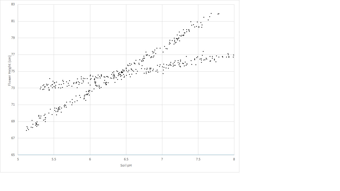
However, I didn't realize when I started my study that the population actually contains two varieties of daffodil, each of which responds very differently to soil pH. So the graph contains two distinct linear relationships:

soil pH vs flower height (cm)

I can eyeball it and separate it manually, of course. But I wonder if there is a more rigorous approach.

Questions:

  1. Is there a statistical test to determine whether a data set would be better fit by a single line or by N lines?

  2. How would I run a linear regression to fit the N lines? In other words, how do I disentangle the co-mingled data?

I can think of some combinatorial approaches, but they seem computationally expensive.


Clarifications:

  1. The existence of two varieties was unknown at the time of data collection. The variety of each daffodil was not observed, not noted, and not recorded.

  2. It is impossible to recover this information. The daffodils have died since the time of data collection.

I have the impression that this problem is something similar to applying clustering algorithms, in that you almost need to know the number of clusters before you start. I believe that with ANY data set, increasing the number of lines will decrease the total r.m.s. error. In the extreme, you can divide your data set into arbitrary pairs and simply draw a line through each pair. (E.g., if you had 1000 data points, you could divide them into 500 arbitrary pairs and draw a line through each pair.) The fit would be exact and the r.m.s. error would be exactly zero. But that's not what we want. We want the "right" number of lines.

$\endgroup$
10
  • 1
    $\begingroup$ related stats.stackexchange.com/questions/245902/… $\endgroup$
    – rep_ho
    Commented Jan 28, 2019 at 14:02
  • 3
    $\begingroup$ do you know which dafodil is which varaiety? If so, then you can just include that information into your model $\endgroup$
    – rep_ho
    Commented Jan 28, 2019 at 14:04
  • 1
    $\begingroup$ This seems a classic case of statistical interaction, as in @Demetri Pananos's answer. $\endgroup$
    – rolando2
    Commented Jan 28, 2019 at 15:45
  • 2
    $\begingroup$ I get the feeling that they don't have the information on which variety the flower was in their data. I agree that if they had that then this would just be a case of building an interaction model or even just running separate regressions for each variety. However, if they don't have that info not all hope is lost. One could build a model that estimates not only the separate lines but also predicts the probabilities that each observation belongs to either group. $\endgroup$
    – Dason
    Commented Jan 28, 2019 at 17:01
  • 1
    $\begingroup$ @DemetriPananos I provided an answer that hopefully makes sense. Depending on what they want to do it is quite a bit more work. To do some sort of testing you'd need to do a likelihood ratio test or do some sort of randomization test or something. But they haven't given us too much info and if the goal is just to fit lines and they don't have the labels then it's not too bad to do using the mixtools package. $\endgroup$
    – Dason
    Commented Jan 28, 2019 at 20:32

5 Answers 5

36
$\begingroup$

I think Demetri's answer is a great one if we assume that you have the labels for the different varieties. When I read your question that didn't seem to be the case to me. We can use an approach based on the EM algorithm to basically fit the model that Demetri suggests but without knowing the labels for the variety. Luckily the mixtools package in R provides this functionality for us. Since your data is quite separated and you seem to have quite a bit it should be fairly successful.

library(mixtools)

# Generate some fake data that looks kind of like yours
n1 <- 150
ph1 = runif(n1, 5.1, 7.8)
y1 <- 41.55 + 5.185*ph1 + rnorm(n1, 0, .25)

n2 <- 150
ph2 <- runif(n2, 5.3, 8)
y2 <- 65.14 + 1.48148*ph2 + rnorm(n2, 0, 0.25)

# There are definitely better ways to do all of this but oh well
dat <- data.frame(ph = c(ph1, ph2), 
                  y = c(y1, y2), 
                  group = rep(c(1,2), times = c(n1, n2)))

# Looks about right
plot(dat$ph, dat$y)

# Fit the regression. One line for each component. This defaults
# to assuming there are two underlying groups/components in the data
out <- regmixEM(y = dat$y, x = dat$ph, addintercept = T)

We can examine the results

> summary(out)
summary of regmixEM object:
          comp 1    comp 2
lambda  0.497393  0.502607
sigma   0.248649  0.231388
beta1  64.655578 41.514342
beta2   1.557906  5.190076
loglik at estimate:  -182.4186 

So it fit two regressions and it estimated that 49.7% of the observations fell into the regression for component 1 and 50.2% fell into the regression for component 2. The way I simulated the data it was a 50-50 split so this is good.

The 'true' values I used for the simulation should give the lines:

y = 41.55 + 5.185*ph and y = 65.14 + 1.48148*ph

(which I estimated 'by hand' from your plot so that the data I create looks similar to yours) and the lines that the EM algorithm gave in this case were:

y = 41.514 + 5.19*ph and y = 64.655 + 1.55*ph

Pretty darn close to the actual values.

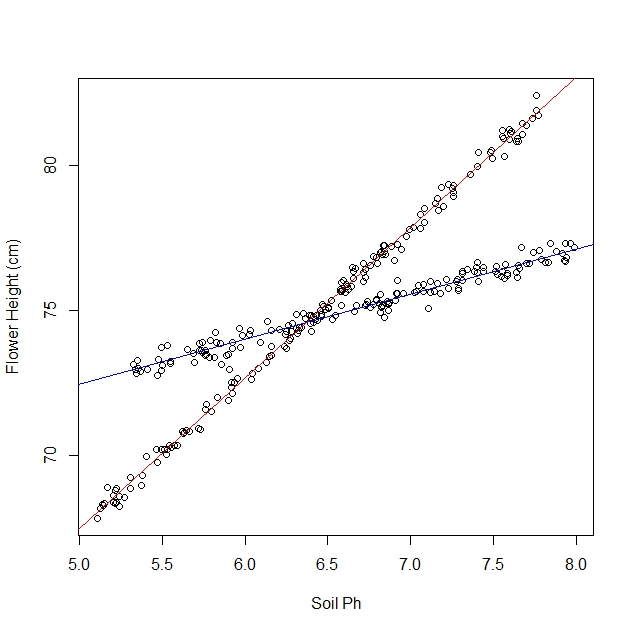
We can plot the fitted lines along with the data

plot(dat$ph, dat$y, xlab = "Soil Ph", ylab = "Flower Height (cm)")
abline(out$beta[,1], col = "blue") # plot the first fitted line
abline(out$beta[,2], col = "red") # plot the second fitted line

Fitted lines via EM

$\endgroup$
22
$\begingroup$

EDIT: I originally thought OP knew which observations came from which species. OP's edit makes it clear that my original approach is not feasible. I'll leave it up for posterity, but the other answer is much better. As a consolation, I've coded up a mixture model in Stan. I'm not saying a Bayesian approach is particularly good in this case, but it is just something neat I can contribute.

Stan Code

data{

  //Number of data points
  int N; 

  real y[N];
  real x[N];
}
parameters{
  //mixing parameter
  real<lower=0, upper =1>  theta;

  //Regression intercepts
  real beta_0[2];

  //Regression slopes.
  ordered[2] beta_1;

  //Regression noise
  real<lower=0> sigma[2];
}
model{

  //priors
  theta ~ beta(5,5);
  beta_0 ~ normal(0,1);
  beta_1 ~ normal(0,1);
  sigma ~ cauchy(0,2.5);

  //mixture likelihood
  for (n in 1:N){
    target+=log_mix(theta,
                     normal_lpdf(y[n] | beta_0[1] + beta_1[1]*x[n], sigma[1]),
                     normal_lpdf(y[n] | beta_0[2] + beta_1[2]*x[n], sigma[2]));
  }
}
generated quantities {
  //posterior predictive distribution
  //will allow us to see what points belong are assigned
  //to which mixture 
  matrix[N,2] p;
  matrix[N,2] ps;
  for (n in 1:N){
    p[n,1] = log_mix(theta,
                     normal_lpdf(y[n] | beta_0[1] + beta_1[1]*x[n], sigma[1]),
                     normal_lpdf(y[n] | beta_0[2] + beta_1[2]*x[n], sigma[2]));

    p[n,2]= log_mix(1-theta,
                     normal_lpdf(y[n] | beta_0[1] + beta_1[1]*x[n], sigma[1]),
                     normal_lpdf(y[n] | beta_0[2] + beta_1[2]*x[n], sigma[2]));

    ps[n,]= p[n,]/sum(p[n,]);
  }
}

Run The Stan Model From R

library(tidyverse)
library(rstan)


#Simulate the data
N = 100
x = rnorm(N, 0, 3)
group = factor(sample(c('a','b'),size = N, replace = T))

y = model.matrix(~x*group)%*% c(0,1,0,2) 
y = as.numeric(y) + rnorm(N)

d = data_frame(x = x, y = y)

d %>% 
  ggplot(aes(x,y))+
  geom_point()

#Fit the model
N = length(x)
x = as.numeric(x)
y = y

fit = stan('mixmodel.stan', 
           data = list(N= N, x = x, y = y),
           chains = 8,
           iter = 4000)

Results

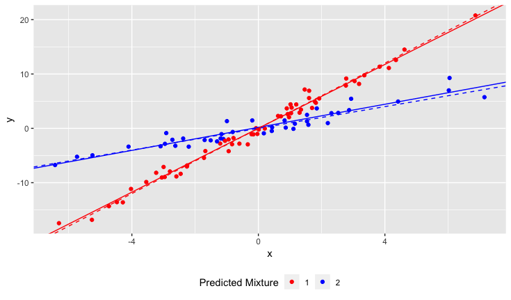
enter image description here

Dashed lines are ground truth, solid lines are estimated.


Original Answer

If you know which sample comes from which variety of daffodil, you can estimate an interaction between variety and soil PH.

Your model will look like

$$ y = \beta_0 + \beta_1 \text{variety} + \beta_2\text{PH} + \beta_3\text{variety}\cdot\text{PH} $$

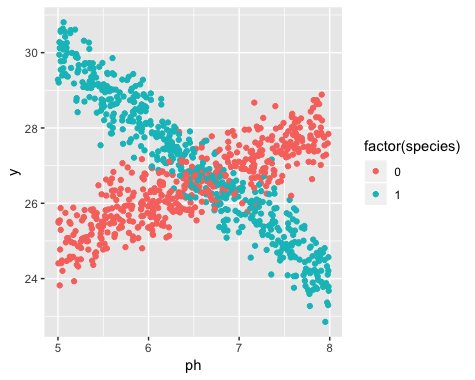
Here is an example in R. I've generated some data that looks like this:

enter image description here

Clearly two different lines, and the lines correspond to two species. Here is how to estimate the lines using linear regression.

library(tidyverse)

#Simulate the data
N = 1000
ph = runif(N,5,8)
species = rbinom(N,1,0.5)

y = model.matrix(~ph*species)%*% c(20,1,20,-3) + rnorm(N, 0, 0.5)
y = as.numeric(y)

d = data_frame(ph = ph, species = species, y = y)

#Estimate the model
model = lm(y~species*ph, data = d)
summary(model)

And the result is

> summary(model)

Call:
lm(formula = y ~ species * ph, data = d)

Residuals:
     Min       1Q   Median       3Q      Max 
-1.61884 -0.31976 -0.00226  0.33521  1.46428 

Coefficients:
            Estimate Std. Error t value Pr(>|t|)    
(Intercept) 19.85850    0.17484  113.58   <2e-16 ***
species     20.31363    0.24626   82.49   <2e-16 ***
ph           1.01599    0.02671   38.04   <2e-16 ***
species:ph  -3.03174    0.03756  -80.72   <2e-16 ***
---
Signif. codes:  
0 ‘***’ 0.001 ‘**’ 0.01 ‘*’ 0.05 ‘.’ 0.1 ‘ ’ 1

Residual standard error: 0.4997 on 996 degrees of freedom
Multiple R-squared:  0.8844,    Adjusted R-squared:  0.8841 
F-statistic:  2541 on 3 and 996 DF,  p-value: < 2.2e-16

For species labeled 0, the line is approximately

$$ y = 19 + 1\cdot \text{PH}$$

For species labeled 1, the line is approximately

$$ y = 40 - 2 \cdot \text{PH} $$

$\endgroup$
4
  • $\begingroup$ If OP knows variety of daffodil in advance, why can't they just split the data in two parts, and run two separate regressions for each variety? $\endgroup$
    – Akavall
    Commented Jan 28, 2019 at 20:50
  • $\begingroup$ If OP isn't interested in differences between daffodil varieties (e.g. Does variety 1 grow taller than variety 2 conditioned on soil PH) then there is no reason to regress all the data together, except for maybe arguments surrounding precision. $\endgroup$ Commented Jan 28, 2019 at 21:10
  • $\begingroup$ @Akavail - They could split the data but running it like this does make it easier to do any sort of comparisons if they were interested in testing any hypothesis about differences between the varieties. Running it combined would also give slightly better estimates if an equal variance assumption is valid. $\endgroup$
    – Dason
    Commented Jan 28, 2019 at 21:16
  • 1
    $\begingroup$ Before I looked into the EM approach I considered the Bayesian approach. But as much as I like the bayesian way of doing things I got lazy and it's much easier to just take the EM approach. With that said I much prefer a Bayesian analysis and I think it makes answering follow up questions much easier as well - you may have a harder time coding the initial model up but once you do it's a lot easier to answer questions you might have using the posterior distribution. $\endgroup$
    – Dason
    Commented Jan 29, 2019 at 22:01
2
$\begingroup$

The statistical approach is very similar to two of the answer above, but it deals a bit more with how to pick the number of latent classes if you lack prior knowledge. You can use information criteria or parsimony as a guide in choosing number of latent classes.

Here is a Stata example using a sequence of finite mixture models (FMMs) with 2-4 latent classes/components. The first table is the coefficients for the latent class membership. These are a bit difficult to interpret, but they can be converted to probabilities later with estat lcprob. For each class, you also get an intercept and a ph slope parameter, followed by latent class marginal probabilities, and two in-sample ICs. These coefficient estimates are interpreted just as the coefficients from a linear regression model. Here the smallest in-sample BIC tells you to pick the two component model as the best one. AIC strangely selects the 3 component model. You can also use out-of-sample ICs to pick or use cross validation.

Another way to gauge that you are pushing the data too far is if the last class share is very small, since an additional components may simply reflect the presence of outliers in the data. In that case, parsimony favors simplifying the model and removing components. However, if you think that small classes are possible in your setting, this may not be the canary in the coal mine. Here parsimony favors the 2 component model since the third class only contains $.0143313 \cdot 300 \approx 4$ observations.

The FMM approach will not always work this well in practice if the classes are less stark. You may run into computational difficulties with too many latent classes, especially if you don't have enough data, or the likelihood function has multiple local maxima.

. clear

. /* Fake Data */
. set seed 10011979

. set obs 300
number of observations (_N) was 0, now 300

. gen     ph = runiform(5.1, 7.8) in 1/150
(150 missing values generated)

. replace ph = runiform(5.3, 8)   in 151/300
(150 real changes made)

. gen y      = 41.55 + 5.185*ph   + rnormal(0, .25)  in 1/150
(150 missing values generated)

. replace y  = 65.14 + 1.48148*ph + rnormal(0, 0.25) in 151/300
(150 real changes made)

. 
. /* 2 Component FMM */
. fmm 2, nolog: regress y ph

Finite mixture model                            Number of obs     =        300
Log likelihood =  -194.5215

------------------------------------------------------------------------------
             |      Coef.   Std. Err.      z    P>|z|     [95% Conf. Interval]
-------------+----------------------------------------------------------------
1.Class      |  (base outcome)
-------------+----------------------------------------------------------------
2.Class      |
       _cons |   .0034359   .1220066     0.03   0.978    -.2356927    .2425645
------------------------------------------------------------------------------

Class          : 1
Response       : y
Model          : regress

------------------------------------------------------------------------------
             |      Coef.   Std. Err.      z    P>|z|     [95% Conf. Interval]
-------------+----------------------------------------------------------------
y            |
          ph |   5.173137   .0251922   205.35   0.000     5.123761    5.222513
       _cons |     41.654   .1622011   256.80   0.000      41.3361    41.97191
-------------+----------------------------------------------------------------
     var(e.y)|   .0619599   .0076322                      .0486698     .078879
------------------------------------------------------------------------------

Class          : 2
Response       : y
Model          : regress

------------------------------------------------------------------------------
             |      Coef.   Std. Err.      z    P>|z|     [95% Conf. Interval]
-------------+----------------------------------------------------------------
y            |
          ph |   1.486062    .026488    56.10   0.000     1.434147    1.537978
       _cons |   65.10664   .1789922   363.74   0.000     64.75582    65.45746
-------------+----------------------------------------------------------------
     var(e.y)|   .0630583   .0075271                      .0499042    .0796797
------------------------------------------------------------------------------

. estat lcprob

Latent class marginal probabilities             Number of obs     =        300

--------------------------------------------------------------
             |            Delta-method
             |     Margin   Std. Err.     [95% Conf. Interval]
-------------+------------------------------------------------
       Class |
          1  |    .499141   .0305016      .4396545    .5586519
          2  |    .500859   .0305016      .4413481    .5603455
--------------------------------------------------------------

. estat ic

Akaike's information criterion and Bayesian information criterion

-----------------------------------------------------------------------------
       Model |        Obs  ll(null)  ll(model)      df         AIC        BIC
-------------+---------------------------------------------------------------
           . |        300         .  -194.5215       7     403.043   428.9695
-----------------------------------------------------------------------------
               Note: N=Obs used in calculating BIC; see [R] BIC note.

. 
. /* 3 Component FMM */
. fmm 3, nolog: regress y ph

Finite mixture model                            Number of obs     =        300
Log likelihood =  -187.4824

------------------------------------------------------------------------------
             |      Coef.   Std. Err.      z    P>|z|     [95% Conf. Interval]
-------------+----------------------------------------------------------------
1.Class      |  (base outcome)
-------------+----------------------------------------------------------------
2.Class      |
       _cons |  -.0312504    .123099    -0.25   0.800    -.2725199    .2100192
-------------+----------------------------------------------------------------
3.Class      |
       _cons |  -3.553227   .5246159    -6.77   0.000    -4.581456   -2.524999
------------------------------------------------------------------------------

Class          : 1
Response       : y
Model          : regress

------------------------------------------------------------------------------
             |      Coef.   Std. Err.      z    P>|z|     [95% Conf. Interval]
-------------+----------------------------------------------------------------
y            |
          ph |   5.173077   .0252246   205.08   0.000     5.123637    5.222516
       _cons |   41.65412     .16241   256.48   0.000      41.3358    41.97243
-------------+----------------------------------------------------------------
     var(e.y)|   .0621157   .0076595                      .0487797    .0790975
------------------------------------------------------------------------------

Class          : 2
Response       : y
Model          : regress

------------------------------------------------------------------------------
             |      Coef.   Std. Err.      z    P>|z|     [95% Conf. Interval]
-------------+----------------------------------------------------------------
y            |
          ph |   1.476049   .0257958    57.22   0.000      1.42549    1.526608
       _cons |   65.18698   .1745018   373.56   0.000     64.84496    65.52899
-------------+----------------------------------------------------------------
     var(e.y)|   .0578413   .0070774                      .0455078    .0735173
------------------------------------------------------------------------------

Class          : 3
Response       : y
Model          : regress

------------------------------------------------------------------------------
             |      Coef.   Std. Err.      z    P>|z|     [95% Conf. Interval]
-------------+----------------------------------------------------------------
y            |
          ph |   1.776746   .0020074   885.09   0.000     1.772811     1.78068
       _cons |   62.76633   .0134072  4681.54   0.000     62.74005    62.79261
-------------+----------------------------------------------------------------
     var(e.y)|   9.36e-06   6.85e-06                      2.23e-06    .0000392
------------------------------------------------------------------------------

. estat lcprob

Latent class marginal probabilities             Number of obs     =        300

--------------------------------------------------------------
             |            Delta-method
             |     Margin   Std. Err.     [95% Conf. Interval]
-------------+------------------------------------------------
       Class |
          1  |   .5005343   .0304855      .4410591    .5599944
          2  |   .4851343   .0306119      .4256343    .5450587
          3  |   .0143313   .0073775      .0051968     .038894
--------------------------------------------------------------

. estat ic

Akaike's information criterion and Bayesian information criterion

-----------------------------------------------------------------------------
       Model |        Obs  ll(null)  ll(model)      df         AIC        BIC
-------------+---------------------------------------------------------------
           . |        300         .  -187.4824      11    396.9648   437.7064
-----------------------------------------------------------------------------
               Note: N=Obs used in calculating BIC; see [R] BIC note.

. 
. /* 4 Component FMM */
. fmm 4, nolog: regress y ph

Finite mixture model                            Number of obs     =        300
Log likelihood = -188.06042

------------------------------------------------------------------------------
             |      Coef.   Std. Err.      z    P>|z|     [95% Conf. Interval]
-------------+----------------------------------------------------------------
1.Class      |  (base outcome)
-------------+----------------------------------------------------------------
2.Class      |
       _cons |  -.6450345   .5853396    -1.10   0.270    -1.792279      .50221
-------------+----------------------------------------------------------------
3.Class      |
       _cons |  -.8026907   .6794755    -1.18   0.237    -2.134438    .5290568
-------------+----------------------------------------------------------------
4.Class      |
       _cons |  -3.484714   .5548643    -6.28   0.000    -4.572229     -2.3972
------------------------------------------------------------------------------

Class          : 1
Response       : y
Model          : regress

------------------------------------------------------------------------------
             |      Coef.   Std. Err.      z    P>|z|     [95% Conf. Interval]
-------------+----------------------------------------------------------------
y            |
          ph |   5.173031   .0251474   205.71   0.000     5.123743    5.222319
       _cons |   41.65574    .161938   257.23   0.000     41.33835    41.97313
-------------+----------------------------------------------------------------
     var(e.y)|   .0617238   .0076596                      .0483975    .0787195
------------------------------------------------------------------------------

Class          : 2
Response       : y
Model          : regress

------------------------------------------------------------------------------
             |      Coef.   Std. Err.      z    P>|z|     [95% Conf. Interval]
-------------+----------------------------------------------------------------
y            |
          ph |   1.503764   .0371216    40.51   0.000     1.431007    1.576521
       _cons |   65.13498   .2666049   244.31   0.000     64.61244    65.65751
-------------+----------------------------------------------------------------
     var(e.y)|   .0387473   .0188853                      .0149062    .1007195
------------------------------------------------------------------------------

Class          : 3
Response       : y
Model          : regress

------------------------------------------------------------------------------
             |      Coef.   Std. Err.      z    P>|z|     [95% Conf. Interval]
-------------+----------------------------------------------------------------
y            |
          ph |   1.441334   .0443892    32.47   0.000     1.354333    1.528335
       _cons |   65.26791   .2765801   235.98   0.000     64.72582       65.81
-------------+----------------------------------------------------------------
     var(e.y)|   .0307352    .010982                      .0152578    .0619127
------------------------------------------------------------------------------

Class          : 4
Response       : y
Model          : regress

------------------------------------------------------------------------------
             |      Coef.   Std. Err.      z    P>|z|     [95% Conf. Interval]
-------------+----------------------------------------------------------------
y            |
          ph |   1.665207   .0079194   210.27   0.000     1.649685    1.680728
       _cons |   63.42577   .0510052  1243.52   0.000      63.3258    63.52573
-------------+----------------------------------------------------------------
     var(e.y)|    .000096   .0000769                        .00002    .0004611
------------------------------------------------------------------------------

. estat lcprob

Latent class marginal probabilities             Number of obs     =        300

--------------------------------------------------------------
             |            Delta-method
             |     Margin   Std. Err.     [95% Conf. Interval]
-------------+------------------------------------------------
       Class |
          1  |   .4991443   .0304808      .4396979     .558615
          2  |   .2618733   .1506066      .0715338    .6203076
          3  |   .2236773    .150279      .0501835    .6110804
          4  |    .015305    .008329       .005234    .0438994
--------------------------------------------------------------

. estat ic

Akaike's information criterion and Bayesian information criterion

-----------------------------------------------------------------------------
       Model |        Obs  ll(null)  ll(model)      df         AIC        BIC
-------------+---------------------------------------------------------------
           . |        300         .  -188.0604      15    406.1208   461.6776
-----------------------------------------------------------------------------
               Note: N=Obs used in calculating BIC; see [R] BIC note.
$\endgroup$
1
  • $\begingroup$ Thank you for this very interesting answer. You have given me some new concepts to research! $\endgroup$
    – SlowMagic
    Commented Jan 29, 2019 at 16:46
0
$\begingroup$

I'll focus on the question of statistical significance since Dason already covered the modeling part.

I am unfamiliar with any formal tests for this (which I am sure exist), so I'll just throw some ideas out there (and I'll probably add R code and technical details later).

First, it is convenient to infer the classes. Presuming you have two lines fit to the data, you can approximately reconstruct the two classes by assigning each point to the class of the line closest to it. For points near the intersection, you will run into issues, but for now just ignore those (there may be a way to get around this, but for now just hope that this won't change much).

The way to do this is to choose $x_{l}$ and $x_{r}$ (soil pH values) with $x_{l} \leq x_{r}$ such that the parts left of $x_{l}$ are sufficiently separated and the parts right of $x_{r}$ are sufficiently separated (the closest point where the distributions don't overlap).

Then there are two natural ways I see to go about doing this.

The less fun way is to just run your original dataset combined with the inferred class labels through a linear regression as in Demetri's answer.

A more interesting way to do so would be through a modified version of ANOVA. The point is to create an artificial dataset that represents the two lines (with similar spread between them) and then apply ANOVA. Technically, you need to do this once for the left side, and once for the right (i.e. you'll have two artificial datasets).

We start with the left, and apply a simple averaging approach to get two groups. Basically, each point in say the first class is of the form $$ y^{(i)}_{1} = \beta_{1,1} x_{1}^{(i)} + \beta_{1,0} + e_{1}^{(i)}$$ so we are going to replace the linear expression $\beta_{1,1} x_{1}^{(i)} + \beta_{1,0}$ by a constant, namely the average value of the linear term or $$ \beta_{1,1} x^{\mathrm{avg}} + \beta_{1, 0}$$ where $x^{\mathrm{avg}}_{l}$ is literally the average $x$ value for the left side (importantly, this is over both classes, since that makes things more consistent). That is, we replace $y_{1}^{(i)}$ with $$ \tilde{y}_{1}^{(i)} = \beta_{1,1} x^{\mathrm{avg}} + \beta_{1, 0} + e_{1}^{(i)},$$ and we similarly for the second class. That is, your new dataset consists of the collection of $\tilde{y}_{1}^{(i)}$ and similarly $\tilde{y}_{2}^{(i)}$.

Note that both approaches naturally generalize to $N$ classes.

$\endgroup$
-2
$\begingroup$

Is it possible that including both in the same chart is an error? Given that the varieties behave completely different is there any value in overlapping the data? It seems to me that you are looking for impacts to a species of daffodil, not the impacts of similar environments on different daffodils. If you have lost the data that helps determine species "A" from species "B" you can simply group behavior "A" and behavior "B" and include the discovery of two species in your narrative. Or, if you really want one chart, simply use two data sets on the same axis. I don't have anywhere near the expertise that I see in the other responses given so I have to find less "skilled" methods. I would run a data analysis in a worksheet environment where the equations are easier to develop. Then, once the groupings become obvious, create the two separate data tables followed by converting them into charts/graphs. I work with a great deal of data and I often find that my assumptions of differing correlations turn out wrong; that is what data is supposed to help us discover. Once I learn that my assumptions are wrong, I display the data based upon the behaviors discovered and discuss those behaviors and resulting statistical analyses as part of the narrative.

$\endgroup$
2
  • 1
    $\begingroup$ I am surmising that you have been downvoted because your answer is not providing any clarity or insight in response to the question. You need to structure your answer more helpfully and make clear what sub-questions you address at each point. The question was updated between answers and before your answer to clearly state that the variety info was not available not recoverable. $\endgroup$
    – ReneBt
    Commented Jan 29, 2019 at 10:32
  • 2
    $\begingroup$ Welcome to Cross Validated! Please don't be put off by your first answer's not being well received - & simpler solutions can be very useful - but as the questioner already states "I can eyeball it and separate it manually, of course", it doesn't seem to be adding much. $\endgroup$
    – Scortchi
    Commented Jan 29, 2019 at 10:34

Your Answer

By clicking “Post Your Answer”, you agree to our terms of service and acknowledge you have read our privacy policy.

Not the answer you're looking for? Browse other questions tagged or ask your own question.