Removal of partitioning variable in final glmtree with new (unused) partitioner -- why?

Question

I'm modeling the likelihood of forest recovery from fire (data here), using glmtrees from the partykit package. I'm quite new to this approach and CV, so I appreciate any guidance. (I think this question fits here in CV as it's about interpreting statistical results...)

I'd like to understand why adding a new possible partitioning variable in my glmtree formula seemingly removes another partitioner from the final tree, even though that new one is not included in the final tree. This first tree does NOT use def59_z_13 as a possible partitioner and here's the result:

tree.mob.pipo.v1 <- glmtree(regen_pipo ~ YEAR.DIFF
                     | BALive_pipo + BALiveTot 
                     + CMD_1995 + MAP_1995
                     + REBURN
                     + FIRE.SEV,
                     data = data.pipo, 
                     family = binomial(link = "logit"),
                     minsplit = 50)

...but including def59_z_13 suggests that FIRE.SEV is no longer an important partitioning variable:

tree.mob.pipo.v2 <- glmtree(regen_pipo ~ YEAR.DIFF
                     | BALive_pipo + BALiveTot 
                     + CMD_1995 + MAP_1995
                     + def59_z_13
                     + REBURN
                     + FIRE.SEV,
                     data = data.pipo, 
                     family = binomial(link = "logit"),
                     minsplit = 50).

FIRE.SEV and def59_z_13 are not well correlated so why does adding def59_z_13 suddenly make FIRE.SEV less significant in my model? Shouldn't the instability associated with FIRE.SEV remain the same such that there's still a break-point in FIRE.SEV?

Thanks for any thoughts!

Answer 1

The model-based recursive partitioning algorithm (MOB) decides in each step whether the parameters of the model are stable across the partitioning variables or whether there is a significant instability. If there is, then the variable with the highest instability (= lowest p-value) is selected for splitting the data/model. Then the procedure is repeated recursively until there are no more significant instabilities or another stopping criterion (like the minimal sample size, maximum depth, etc.) is met.

To avoid splitting on spuriously significant variables, MOB by default uses a Bonferroni correction for the p-values from the tests for each partitioning variables. Thus, when testing only a single partitioning variable, the p-value has to be lower than 5% (by default) to be significant. If two variables are tested, the unadjusted p-value would have to be lower than approximately 2.5%, etc.

Therefore, the test statistic of FIRE.SEV and corresponding unadjusted p-value does not change at all when def59_z_13 is included as a potential partitioning variable. However, the adjusted p-value increases because more potential partitioning variables are assessed. To see this check:

library("strucchange")
sctest(tree.mob.pipo.v1, node = 2)
##           BALive_pipo BALiveTot CMD_1995 MAP_1995 REBURN FIRE.SEV
## statistic       3.405    7.2509   4.4042    3.304 4.2456  15.8684
## p.value         1.000    0.8647   0.9989    1.000 0.5346   0.0497
sctest(tree.mob.pipo.v2, node = 2)
##           BALive_pipo BALiveTot CMD_1995 MAP_1995 def59_z_13 REBURN FIRE.SEV
## statistic       3.405    7.2509   4.4042    3.304     4.2576 4.2456 15.86841
## p.value         1.000    0.9031   0.9997    1.000     0.9998 0.5903  0.05774

Thus, with only six partitioning variable, the adjusted p-value is 4.97% and just significant. With seven partitioning variables, it turns non-significant due to the Bonferroni adjustment.

So one could think you would have to be forced to decide how much p-hacking you are willing to do here... Fortunately, there is a better solution. The FIRE.SEV variable was treated as continuous but it would be much more appropriate to treat it as ordinal and employ the dedicated ordinal statistic of Merkle et al. (2014). "Testing for Measurement Invariance with Respect to an Ordinal Variable." Psychometrika, 79(4), 569-584. doi:10.1007/S11336-013-9376-7.

data.pipo <- read.csv("https://raw.githubusercontent.com/CaitLittlef/fia-regen/master/data.pipo.share.csv")
data.pipo <- transform(data.pipo,
  regen_pipo = factor(regen_pipo),
  FIRE.SEV = factor(FIRE.SEV, ordered = TRUE)
)
tree.pipo <- glmtree(regen_pipo ~ YEAR.DIFF | BALive_pipo +
  BALiveTot + CMD_1995 + MAP_1995 + def59_z_13 + REBURN + FIRE.SEV,
  data = data.pipo, family = binomial, minsplit = 50, ordinal = "L2")
sctest(tree.pipo, node = 2)
##           BALive_pipo BALiveTot CMD_1995 MAP_1995 def59_z_13 REBURN FIRE.SEV
## statistic       3.405    7.2509   4.4042    3.304     4.2576 4.2456 12.96481
## p.value         1.000    0.9031   0.9997    1.000     0.9998 0.5903  0.03568

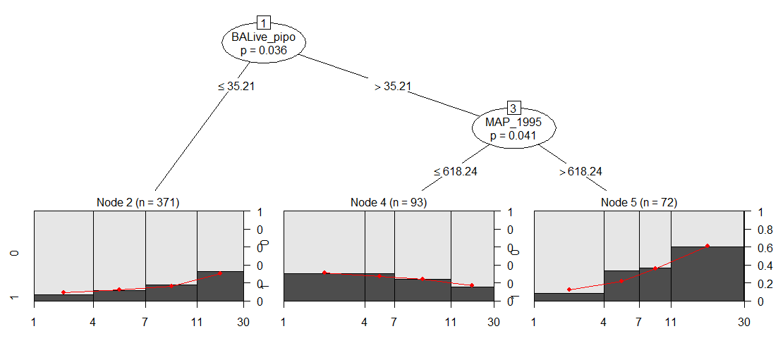
Thus, this yields the same tree as your v1 and the p-value is still somewhat smaller with 3.6%.