Posterior predictive distributions and predictive intervals

Question

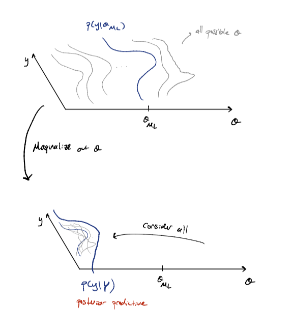
I'm confused about the role of posterior predictive distributions in Bayesian inference and predictive inference.

As I understand it, the frequentist approach would typically involve fitting the MLE, which would return a single estimate of the parameter set for the data - so there is a single distribution for predicting new data points.

As I understand it, in Bayesian inference, the posterior predictive distribution is the probability distribution of a new data point, as opposed to the posterior distribution which is a distribution of the parameter. However, to obtain the posterior predictive distribution, you marginalise over the parameter by integrating over it.

$p(\tilde{x}|\alpha )=\int p(\tilde{x}|\theta ) p(\theta |\alpha )d\theta$

Each possible value of $\theta$ would give you a different distribution. Marginalising is (broadly) equivalent to taking a weighted average over the uncertainty in the parameter e.g. averaging over all the distributions that would arise from each possible value of the $\theta$, weighted by the probability of that $\theta$. If we imagine the levels within a Bayesian model (from $\alpha$ to $\theta$ to observations) then are we essentially averaging out over that middle layer?

If so, does this not also result in a single distribution for predicting new data points, just one that has accounted for the uncertainty while being determined? Does this not discard (or at least, use and then discard) useful information?

I am struggling to wrap my head around how this links to some other aspects/applications of Bayesian inference - which makes me suspect that I've misunderstood something.

1. Prediction intervals: I thought that one of the key advantages of Bayesian inference is that it enabled easier quantification of prediction intervals, which might be needed depending on how the prediction is being used (e.g. what if we are interested in the 95th or 99th quantile of the prediction interval). But by marginalising over $\theta$, have we not lost the information that would have enabled that? I have seen some discussion of posterior predictive intervals, but I don't really understand.

2. Bayesian neural networks: Similar to the above, I thought that the key advantage of BNNs is that they allow for the quantification of uncertainty. Would marginalising over the parameters not collapse this uncertainty?

3. Hierarchical models: If you are trying to predict a new, unknown, group within a hierarchical model, then it seems to me that you'd want to keep the quantified uncertainty (reflecting you don't know exactly the characteristics of this new group), which would exist in the variance of the second level of the model. Would marginalising for the posterior predictive require you to integrate away this (potentially insightful) uncertainty? Or do you only marginalise over the parameter uncertainty?

Answer 1

"But by marginalising over 𝜃 , have we not lost the information that would have enabled that?"

I'll try and provide insight into why the answer to this is no.

If we were to consider the parameters $\theta$ as a single point, we could fit a model (for example) via maximum likelihood estimation to yield

$$ p(y|\theta_{\text{ML}}) $$

Realize that we simply ignore the idea that there is randomness in $\theta$. In a Bayesian treatment, we don't ignore this, and we instead seek to find a distribution over $\theta$ rather than a point estimate for $\theta$. The distribution that takes into account the observed dataset we have at hand is called the "posterior" and I will denote it as $p(\theta|\pmb{\mathsf{y}})$.

Then, if we are interested in prediction, we compute the posterior predictive by marginalizing over all possible settings of $\theta$ contained in the posterior $p(\theta|\pmb{\mathsf{y}})$:

$$ p(y|\pmb{\mathsf{y}}) = \int p(y|\theta)p(\theta|\pmb{\mathsf{y}}) \text{d}\theta $$

The MLE fitted model $p(y| \theta_{\text{ML}})$ considers a fixed $\theta$ and looks at the distribution over $y$ given such a fixed setting of $\theta$.

The Bayesian posterior predictive $p(y|\pmb{\mathsf{y}})$ considers a random $\theta$ and looks at the distribution over $y$ after considering all possible $\theta$ as per the posterior. Intuitively, it should have "more randomness" or "uncertainty" and it does. Namely, it has introduced "model" or "epistemic" uncertainty -- uncertainty coming from many different settings of $\theta$ that induce a model $p(y|\theta)$ that can explain our dataset at hand.

The variance of $p(y|\pmb{\mathsf{y}})$ will necessarily be greater than or equal to $p(y|\theta_{\text{ML}})$. Maybe the (very simplified) visualization below can help

Also see Pattern Recognition and Machine Learning (Chris M. Bishop) https://www.microsoft.com/en-us/research/uploads/prod/2006/01/Bishop-Pattern-Recognition-and-Machine-Learning-2006.pdf. Specifically, section 1.2.5.