Manual simulation of Markov Chain in R

Question

Consider the Markov chain with state space S = {1, 2}, transition matrix

and initial distribution α = (1/2, 1/2).

1. Simulate 5 steps of the Markov chain (that is, simulate X₀, X₁, . . . , X₅). Repeat the simulation 100 times. Use the results of your simulations to solve the following problems.

   • Estimate P(X₁ = 1|X₀ = 1). Compare your result with the exact probability.

My solution:

# returns Xn 
func2 <- function(alpha1, mat1, n1) 
{
  xn <- alpha1 %*% matrixpower(mat1, n1+1)

  return (xn)
}

alpha <- c(0.5, 0.5)
mat <- matrix(c(0.5, 0.5, 0, 1), nrow=2, ncol=2)
n <- 10


for (variable in 1:100) 
{
   print(func2(alpha, mat, n))
}

What is the difference if I run this code once versus 100 times (as is said in the problem-statement)?

How can I find the conditional probability from here on?

Answer 1

The R function func2 produces the vector$$(\alpha,1-\alpha) \mathbf P^n$$which is the marginal distribution of the Markov chain after $n$ steps, given that the initial state is generated with distribution $(\alpha,1-\alpha)$. To generate the Markov chain, one needs to proceed one step at a time:

1. generate $X_0$ equal to $1$ with probability $\alpha$ and $2$ with probability $1-\alpha$
2. generate $X_1$ which is equal to $2$ if $X_0=2$ and to $1$ with probability $1/2$ and $2$ with probability $1/2$ if $X_0=1$
3. generate $X_2$ which is equal to $2$ if $X_1=2$ and to $1$ with probability $1/2$ and $2$ with probability $1/2$ if $X_1=1$
4. generate $X_3$ which is equal to $2$ if $X_2=2$ and to $1$ with probability $1/2$ and $2$ with probability $1/2$ if $X_2=1$
5. generate $X_4$ which is equal to $2$ if $X_3=2$ and to $1$ with probability $1/2$ and $2$ with probability $1/2$ if $X_3=1$
6. generate $X_5$ which is equal to $2$ if $X_4=2$ and to $1$ with probability $1/2$ and $2$ with probability $1/2$ if $X_4=1$

Each transition can be simulated by a one-line code such as

tranz <- function(x=1) 2-(x==1)*(runif(1)<.5)

leading to a five step Markov chain in a similarly easy coding such as

marx <- function(alf=.5){ 
   x=2-(runif(1)<alf)
   for (t in 2:6) x=c(x,tranz(x[t-1]))
   return(x)}

Thus one recovers one realisation of the sequence $X_0,X_1,X_2,X_3,X_4,X_5$. Rerunning the algorithm 99 times produces in total 100 realisations of the sequence $X_0,X_1,X_2,X_3,X_4,X_5$. Not necessarily all different (actually certainly not all different!), but iid replicas of such realisations, from which $\mathbb P(X_1 = 1|X_0 = 1)$ and $\mathbb P(X_5 = 1|X_0 = 1)$ can be estimated by the Law of Large Numbers.

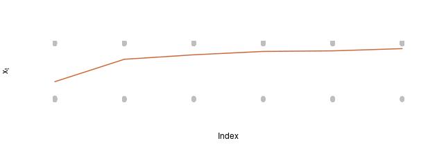
Here is an illustration for 100 replications when $\alpha=.7$:

where the 6x100 values have been jittered and the curve corresponds to the 6 means of the simulated $X_t$'s.