estimate confidence interval of empirical percentile [duplicate]

Question

Suppose $n$ samples are generated from an unknown distributions and the empirical percentile is estimated.

In python:

import numpy as np
n_samples = 30
desired_percentile = 90
x = np.random.uniform(0, 1, n_samples) # data from an unknown distribution
perc = np.percentile(x, desired_percentile)

How can I estimate how close my estimated percentile is to the real percentile of the distribution?

I would like to estimate something like $p=P(|perc- real~perc| > \delta)$ that in this example is equivalent to $P(|perc-0.9|>\delta)$.

Note that in general the $real~perc$ value is not known and that I expect $p \rightarrow 0 ~if ~ n \rightarrow\infty$

UPDATE 1

All the answers at the moment seems to suggest to estimate the confidence interval using bootstrap. Unfortunately bootstrap will work only if enough samples are available.

Suppose using bootstrap we estimate $l$ and $u$ such that:

$P(l < real~perc < p) > 0.9$

this will not take into account the fact that the data is not enough to correctly approximate the original distribution.

Indeed for example in the case of a $n=30$ and $x_i\sim U(0, 1)$ we have:

$P(x_1<0.95,\dots x_n<0.95)=0.21$

as a consequence the $P(l < real~perc < p)$ should be less than $0.79$.

I think an estimate of the CI needs to explicitly take the number of samples $n$ as parameter.

Answer 1

With only $n = 30$ observations, we can't expect any one of the observations to be really close to the 90th percentile of the actual distribution (whatever it may be). Also, if the right tail of the actual distribution is longer it will be harder to find the 90th percentile. Let's try three distributions, and see how well bootstrapping works.

Uniform Data. Suppose the data are from $\mathsf{Unif}(0,100),$ for which $90$ is the 90th percentile. Below we that the 90th percentile of the sample of 30 is $85.3$. Also, 95% of bootstrapped samples had 90th percentiles in the interval $(71.36, 93.79).$ So the bootstrap CI captures what we know in this simulated example to be the true 90th percentile of the population distribution.

set.seed(427)
x = runif(30, 0, 100)  # available sample of 30
quantile(x, .9)
     90% 
85.30419               # 90th percentile of sample

q.boot = replicate(10^5, quantile(sample(x,30,repl=T), .9))
quantile(q.boot, c(.025, .975))
    2.5%    97.5% 
71.36458 93.79138      # quantile boostrap 95% CI

Normal data: If data are from $\mathsf{Norm}(100,10),$ then the true 90th percentile of the population is $112.82.$ The bootstrap CI is $(106.56, 118.10),$

set.seed(428)
qnorm(.9, 100, 10)
[1] 112.8155

The observed 90th percentile from the sample of 30 is 115.86 .

quantile(x, .9)
     90% 
115.8592 

q.boot = replicate(10^5, quantile(sample(x,30,repl=T), .9))          
quantile(q.boot, c(.025, .975))
    2.5%    97.5% 
106.5641 118.0972 

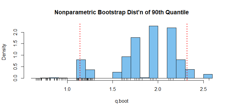
Expontntial data. For a standard exponential distribution (mean = rate = 1), the true 90th percentile is $-\ln(.9) = 2.303.$ A sample of size 30 happens to have a 90th quantile of $1.93.$ The bootstrap Ci is $(1.14, 2.31).$ Relatively speaking, this is the longest interval of the three (upper limit almost double the lower one) because observations are relatively sparse in the long right tail of an exponential distribution.

set.seed(429)
x = rexp(30)
quantile(x, .9)
     90% 
1.934453 

q.boot = replicate(10^5, quantile(sample(x,30,repl=T), .9)) 
quantile(q.boot, c(.025, .975))
    2.5%    97.5% 
1.140935 2.318829 

Of the 100,000 bootstrap re-samples from the exponential sample (each of size 30) there were only 86 uniquely different 90th percentiles. Here is the histogram of the bootstrap distribution. Small tick marks show positions of of the 86 values; some tick marks represent many re-samples with the same 90th percentile. Vertical dotted lines show the limits of the 95% quantile-method bootstrap confidence interval.

Notes: (1) Different software programs have slightly different methods of defining quantiles that can give noticeably different results for small samples. For each original sample the 90th percentile (according to R's default definition), are shown on the respective stripcharts.

(2) For a particular distribution, nonparametric bootstrap procedures based on small samples may give noticeably different results--from one small sample from to another. [Here, seeds are given so you can reproduce the same samples used to get results in the Answer.] As the histogram for the last part (exponential data) shows, bootstrap distributions based on small samples may be discrete in unexpected ways.

(3) There are many different nomparametric bootstrap procedures, various methods may give different results for the same original sample. The method illustrated here is the one of the most elementary.

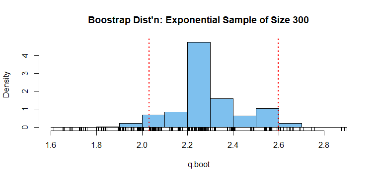
Addendum: We tried the same nonparametric bootstrap method, but using an exponential sample of size $n = 300.$

The bootstrap procedure results in over 300 uniquely different 90th percentiles and the 95% confidence interval $(2.03, 2.60)$--much narrower than for $n=30.$