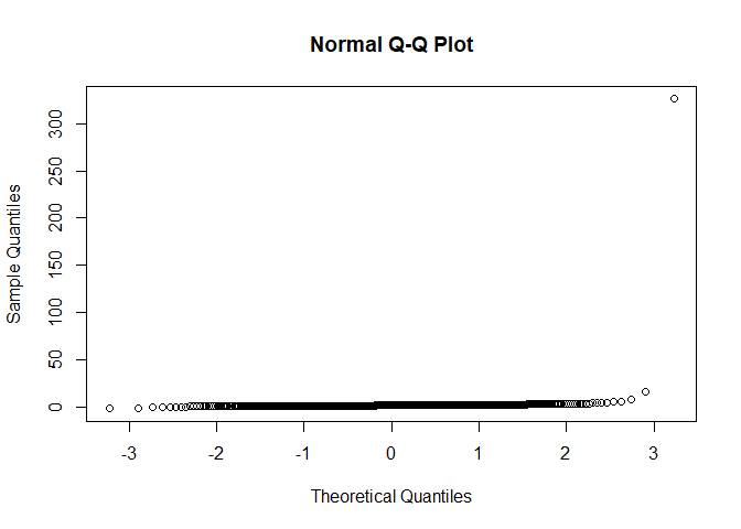
2
$\begingroup$

I have now been studying mixed models for about a month, I am still a pure beginner. I have zero inflated semi continuous dependent variable (yield of trees between two periods). Exploring StackExchange community, there are some questions related to modelling of zero inflated semi continuous data (Zero-inflated two-part models for semi-continuous data; How to model non-negative zero-inflated continuous data?).

But I would like to apply a mixed model to my data and as I can see, this could be done with mixed_model function from the GLMMadaptive R package. There is an example on this link [Two-Part Mixed Effects Model for Semi-Continuous Data].

Ok, let’s go back to my data. I have around 20.000 observations with 8 % of zeros. Brief description of variables:

  1. yield [zero inflated semi continuous variable]
  2. stock [numerical, tree volume in forest]
  3. slope [numerical, slop in forest]
  4. precipitation [numerical, amount of precipitation in growing season]
  5. n_trees [numerical, number of trees in forest]
  6. soil_depth [numerical, soil depth]
  7. rocks [factor, there are five categories, each has different % of rocks covering forest ground]
  8. position [factor, position of a tree in a forest, five categories]
  9. groups [factor with two levels describing trees, conifers and broadleaves]
  10. groups_detailed [factor with 8 levels, similar tree species are in the same group]

My question is related to selection of the best model. If I follow the rule of lowest AIC, I should select the following model:

lowest_AIC <- mixed_model(yield ~ stock, 
                    random = ~  1 | groups, 
                    data = trees, 
                    family = hurdle.lognormal(), n_phis = 1,
                    zi_fixed = ~ stock
)

> AIC(lowest_AIC)
[1] 2784.14
> mean(residuals(lowest_AIC)^2)
[1] 0.1474714
> summary(lowest_AIC)

Call:
mixed_model(fixed = yield ~ stock, random = ~1 | groups, data = trees, 
    family = hurdle.lognormal(), zi_fixed = ~stock, n_phis = 1)

Data Descriptives:
Number of Observations: 20583
Number of Groups: 2 

Model:
 family: hurdle log-normal
 link: identity 

Fit statistics:
  log.Lik     AIC      BIC
 -1386.07 2784.14 2776.299

Random effects covariance matrix:
              StdDev
(Intercept) 1.396311

Fixed effects:
            Estimate Std.Err  z-value p-value
(Intercept)   0.0004  0.0061   0.0731 0.94177
stock        -0.0907  0.0062 -14.7410 < 1e-04

Zero-part coefficients:
            Estimate Std.Err  z-value p-value
(Intercept)  -2.4295  0.0257 -94.3862 < 1e-04
stock         0.1934  0.0238   8.1089 < 1e-04

log(residual std. dev.):
  Estimate Std.Err
   -0.1746  0.0051

Integration:
method: adaptive Gauss-Hermite quadrature rule
quadrature points: 11

Optimization:
method: EM
converged: TRUE 

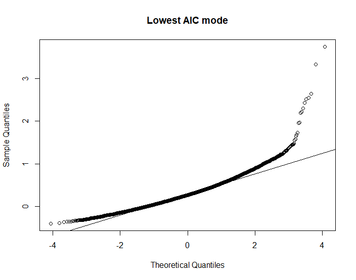
All variables are significant, but qqplot looks bad: enter image description here
Ok, if I experiment further and add some more variables, I end up with the following model:

best <- mixed_model(yield ~ stock + slope + precipitation + n_trees + soil_depth + rocks  + position, 
                    random = ~  1 | groups, 
                    data = trees, 
                    family = hurdle.lognormal(), n_phis = 1, 
                    zi_fixed = ~ stock + slope + precipitation + rocks + position,
                    zi_random = ~  1 | groups

)

> AIC(best)
[1] 2839.902
> mean(residuals(best)^2)
[1] 0.1890385
> summary(best)

Call:
mixed_model(fixed = yield ~ stock + slope + precipitation + n_trees + 
    soil_depth + rocks + position, random = ~1 | groups, data = trees, 
    family = hurdle.lognormal(), zi_fixed = ~stock + slope + 
        precipitation + rocks + position, zi_random = ~1 | groups, 
    n_phis = 1)

Data Descriptives:
Number of Observations: 20528
Number of Groups: 2 

Model:
 family: hurdle log-normal
 link: identity 

Fit statistics:
   log.Lik      AIC      BIC
 -1387.951 2839.902 2798.083

Random effects covariance matrix:
                StdDev    Corr
(Intercept)     1.4117        
zi_(Intercept)  0.1331  0.0477

Fixed effects:
                           Estimate Std.Err  z-value p-value
(Intercept)                  0.4576  0.0176  25.9341 < 1e-04
stock                       -0.0644  0.0059 -10.8639 < 1e-04
slope                       -0.0593  0.0059 -10.1307 < 1e-04
precipitation               -0.0858  0.0061 -14.1035 < 1e-04
n_trees                     -0.0630  0.0060 -10.5368 < 1e-04
soil_depth                   0.0590  0.0061   9.7462 < 1e-04
rocks2                      -0.0847  0.0155  -5.4514 < 1e-04
rocks3                      -0.0942  0.0178  -5.2897 < 1e-04
rocks4                      -0.1437  0.0184  -7.8039 < 1e-04
rocks5                      -0.1933  0.0258  -7.5044 < 1e-04
rocks6                      -0.4962  0.0574  -8.6376 < 1e-04
position-0.561514296868636  -0.2333  0.0180 -12.9644 < 1e-04
position0.381120787744946   -0.4953  0.0193 -25.6413 < 1e-04
position1.32375587235853    -0.8913  0.0234 -38.0653 < 1e-04
position2.26639095697211    -1.0993  0.0276 -39.8970 < 1e-04

Zero-part coefficients:
                           Estimate Std.Err  z-value  p-value
(Intercept)                 -3.5587  0.1180 -30.1541  < 1e-04
stock                        0.1724  0.0255   6.7729  < 1e-04
slope                        0.2517  0.0272   9.2508  < 1e-04
precipitation               -0.1457  0.0296  -4.9197  < 1e-04
rocks2                       0.3587  0.0719   4.9900  < 1e-04
rocks3                       0.3497  0.0823   4.2506  < 1e-04
rocks4                       0.3951  0.0845   4.6742  < 1e-04
rocks5                       0.5387  0.1110   4.8507  < 1e-04
rocks6                       0.5434  0.2539   2.1404 0.032319
position-0.561514296868636   0.3085  0.1215   2.5384 0.011136
position0.381120787744946    0.8707  0.1219   7.1406  < 1e-04
position1.32375587235853     1.5953  0.1251  12.7515  < 1e-04
position2.26639095697211     2.0707  0.1270  16.3061  < 1e-04

log(residual std. dev.):
  Estimate Std.Err
   -0.2856  0.0052

Integration:
method: adaptive Gauss-Hermite quadrature rule
quadrature points: 11

Optimization:
method: hybrid EM and quasi-Newton
converged: TRUE 

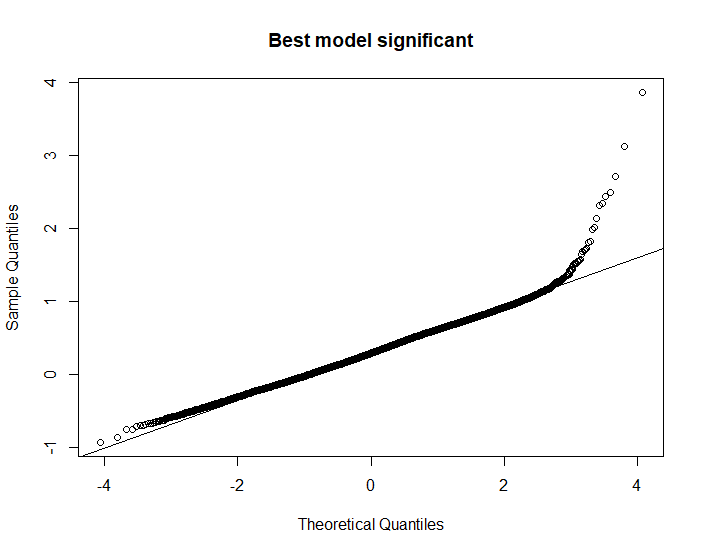
AIC and error is higher, which indicates worse model, but all variables included in this model are significant and qqplot is much better: qqplot for model with more variables
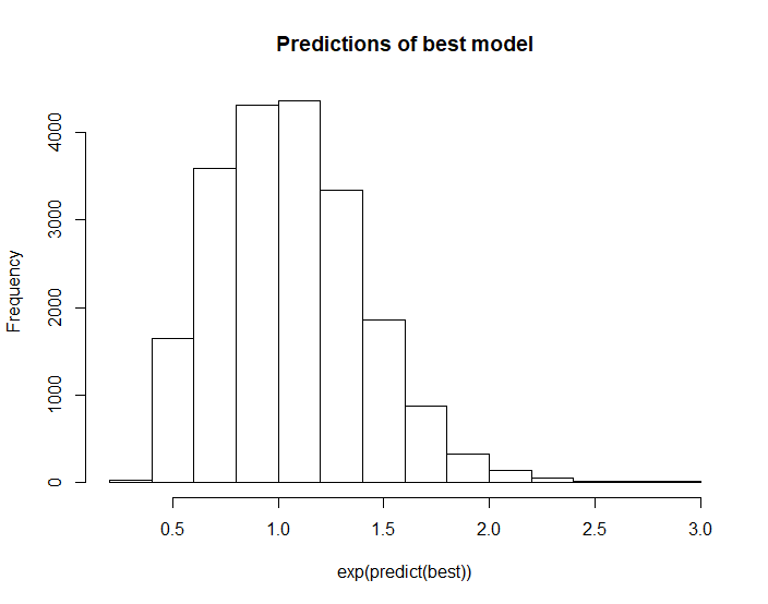
How does AIC relate to significant variables? Should I include those if they are significant even though they increase AIC (and improve qqplot)? I am using Two-Part Mixed Effects Model for Semi-Continuous Data, but zero part does not predict any zero! Here is the plot of predicted yield using best model: enter image description here
What to do? I know some of you might recommend data transformation log(yield + 0.01), but so far this has not turn out to be a good solution.

$\endgroup$

1 Answer 1

4
$\begingroup$

The goodness-of-fit of the model may not be directly related to significance. Actually, it can be that a model that is not appropriate for a particular dataset gives you incorrectly significant results.

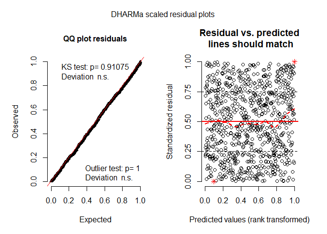
Moreover, for complex models such as this one, it would be better to check the fit using the simulated residuals provided by the DHARMa package instead of the qq-plot. Because the marginal distribution of the data is not normal here due to the extra zeros. For example, check the following code that simulates data from a two-part model, fits the model, and then evaluates the fit (note: it would be best to use the most recent version of GLMMadaptive available from GitHub):

library("GLMMadaptive")
library("DHARMa")
set.seed(1234)
n <- 100 # number of subjects
K <- 8 # number of measurements per subject
t_max <- 5 # maximum follow-up time

# we constuct a data frame with the design: 
# everyone has a baseline measurment, and then measurements at random follow-up times
DF <- data.frame(id = rep(seq_len(n), each = K),
                 time = c(replicate(n, c(0, sort(runif(K - 1, 0, t_max))))),
                 sex = rep(gl(2, n/2, labels = c("male", "female")), each = K))

# design matrices for the fixed and random effects non-zero part
X <- model.matrix(~ sex * time, data = DF)
Z <- model.matrix(~ time, data = DF)
# design matrices for the fixed and random effects zero part
X_zi <- model.matrix(~ sex, data = DF)
Z_zi <- model.matrix(~ 1, data = DF)

betas <- c(-2.13, -0.25, 0.24, -0.05) # fixed effects coefficients non-zero part
sigma <- 0.5 # standard deviation error terms non-zero part
gammas <- c(-1.5, 0.5) # fixed effects coefficients zero part
D11 <- 0.5 # variance of random intercepts non-zero part
D22 <- 0.1 # variance of random slopes non-zero part
D33 <- 0.4 # variance of random intercepts zero part

# we simulate random effects
b <- cbind(rnorm(n, sd = sqrt(D11)), rnorm(n, sd = sqrt(D22)), rnorm(n, sd = sqrt(D33)))
# linear predictor non-zero part
eta_y <- as.vector(X %*% betas + rowSums(Z * b[DF$id, 1:2, drop = FALSE]))
# linear predictor zero part
eta_zi <- as.vector(X_zi %*% gammas + rowSums(Z_zi * b[DF$id, 3, drop = FALSE]))
# we simulate log-normal longitudinal data
DF$y <- exp(rnorm(n * K, mean = eta_y, sd = sigma))
# we set the zeros from the logistic regression
DF$y[as.logical(rbinom(n * K, size = 1, prob = plogis(eta_zi)))] <- 0


km <- mixed_model(y ~ sex * time, random = ~ 1 | id, data = DF, 
                   family = hurdle.lognormal(),
                   zi_fixed = ~ sex, zi_random = ~ 1 | id)


resids_plot <- function (object, y, nsim = 1000,
                         type = c("subject_specific", "mean_subject"),
                         integerResponse = NULL) {
    if (!inherits(object, "MixMod"))
        stop("this function works for 'MixMod' objects.\n")
    type <- match.arg(type)
    if (is.null(integerResponse)) {
        integer_families <- c("binomial", "poisson", "negative binomial",
                              "zero-inflated poisson", "zero-inflated negative binomial", 
                              "hurdle poisson", "hurdle negative binomial")
        numeric_families <- c("hurdle log-normal", "beta", "hurdle beta")
        if (object$family$family %in% integer_families) {
            integerResponse <- TRUE
        } else if (object$family$family %in% numeric_families) {
            integerResponse <- FALSE
        } else {
            stop("non build-in family object; you need to specify the 'integerResponse',\n",
                 "\targument indicating whether the outcome variable is integer or not.\n")
        }
    }
    sims <- simulate(object, nsim = nsim, type = type)
    fits <- fitted(object, type = type)
    dharmaRes <- DHARMa::createDHARMa(simulatedResponse = sims, observedResponse = y, 
                                      fittedPredictedResponse = fits, 
                                      integerResponse = integerResponse)
    DHARMa:::plot.DHARMa(dharmaRes, quantreg = FALSE)
}

# compare the simulated residuals
resids_plot(km, DF$y)

# with the classical QQ-plot
qqnorm(resid(km, type = "subject_specific"))

$\endgroup$
4
  • 3
    $\begingroup$ If the proposed model will be used for prediction, using AIC will make sense. But if the purpose of the model is explanation, BIC could be more appropriate. $\endgroup$ Commented Jun 18, 2019 at 13:06
  • 3
    $\begingroup$ Also, the proposed model makes an assumption that numeric variables such as stock have linear effects, which may not be the case. It’s worth investigating what happens if the linearity assumption is relaxed for such variables (e.g., allow their effects to be nonlinear & smooth) - perhaps the gamlss package in R can handle this. $\endgroup$ Commented Jun 18, 2019 at 13:09
  • 3
    $\begingroup$ @IsabellaGhement You could also add regression splines using, e.g., function ns() from package splines directly into the formulas. $\endgroup$ Commented Jun 18, 2019 at 13:11
  • $\begingroup$ Hi! Thank you very much for this insight. I will come back with feedback after I do my homework. $\endgroup$ Commented Jun 18, 2019 at 13:12

Your Answer

By clicking “Post Your Answer”, you agree to our terms of service and acknowledge you have read our privacy policy.

Not the answer you're looking for? Browse other questions tagged or ask your own question.