I have no formal training in statistics so please correct me if I use the wrong terms as I try to explain my problem.
I have a set of data (less than 80 points) with essentially 1 single outcome (a float we will call dcl) that can potentially depends on 10 of other variables, most of them floats maybe one or two boolean.
While I might ask some multi-variate regression question later, let's start with something simple.
Historically, people in my field have focused on the strongest correlation between dcl and variable J and some of my data suggests some other dependence on a float Re which is I'm sure at least weakly correlated with 'J' as they share some variables in their respective expressions. So my first question is how do I test the correlation and/or the independence of 'Re' and 'J' on the outcome 'dlc'? Intuitively and physically, I expect 'dlc' to depend strongly on 'J' and weakly on 'Re'. How do I prove this with a statistical analysis?
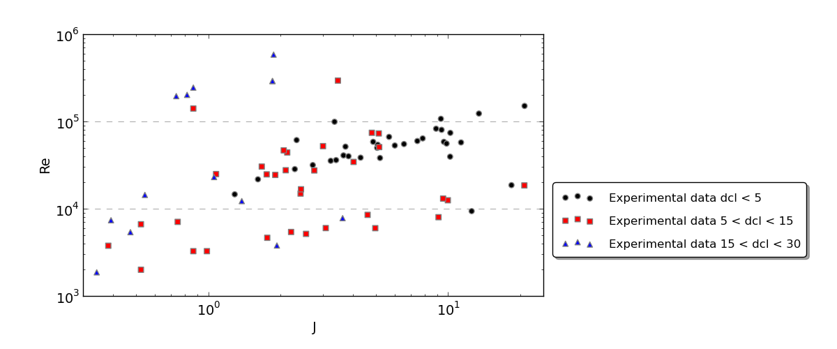
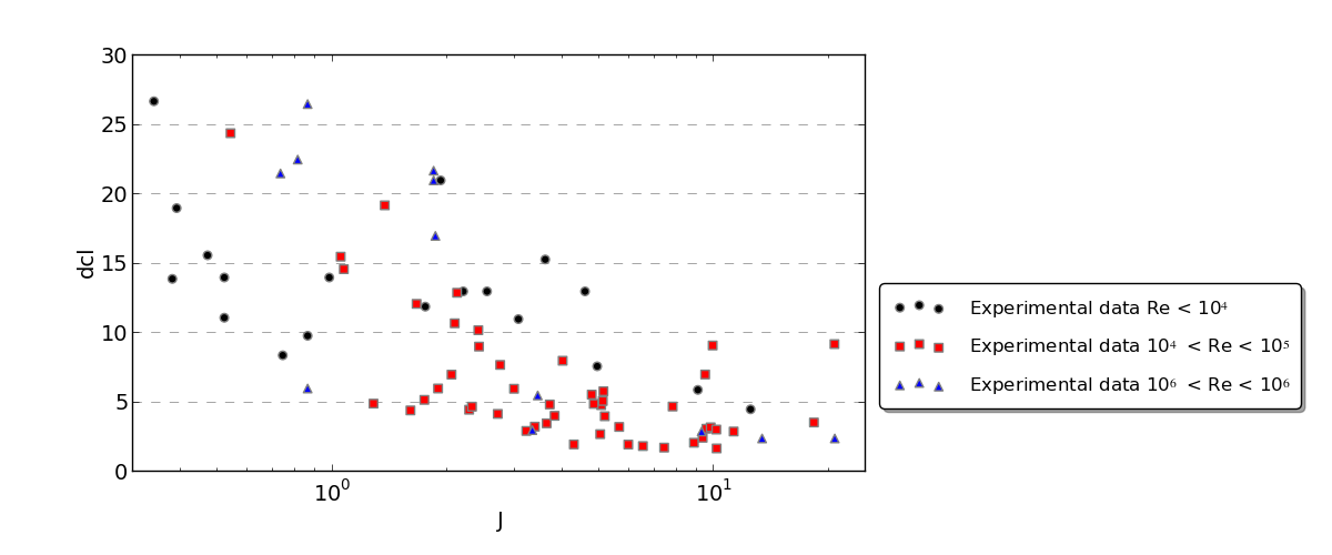
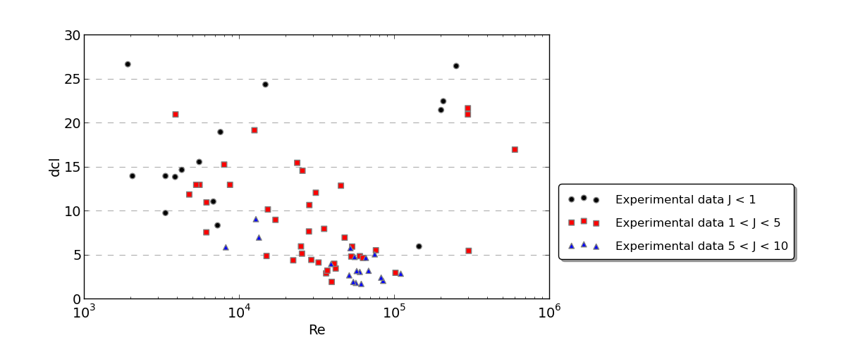
Here are a few graphs to illustrate the data:


Final point, in terms of software, I have python and R installed, I'm fairly proficient in python but I just installed R and know pretty much nothing about it.
EDIT 1:
Following gung's suggestion, I ran my dataset through R:
Call:
lm(formula = dcl ~ J + I(J^2) + Re + I(Re^2), data = df)

Residuals:
    Min      1Q  Median      3Q     Max
-9.0078 -3.7930 -0.4458  2.0869 21.2538

Coefficients:
              Estimate Std. Error t value Pr(>|t|)
(Intercept)  1.648e+01  1.232e+00  13.380  < 2e-16 ***
J           -2.662e+00  3.773e-01  -7.054 6.58e-10 ***
I(J^2)       1.096e-01  2.071e-02   5.293 1.10e-06 ***
Re           1.966e-06  1.621e-05   0.121    0.904
I(Re^2)      2.191e-11  3.441e-11   0.637    0.526
---
Signif. codes:  0 ‘***’ 0.001 ‘**’ 0.01 ‘*’ 0.05 ‘.’ 0.1 ‘ ’ 1

Residual standard error: 5.369 on 77 degrees of freedom
Multiple R-squared: 0.4831, Adjusted R-squared: 0.4562
F-statistic: 17.99 on 4 and 77 DF,  p-value: 1.818e-10
So now I need some help to decipher this (but I will look into R documentation too). I don't know if it's relevant but on physical grounds only, it's probable the dependency in J is $dcl \sim \frac{1}{\sqrt{J}}$. Can I put this directly into the model? Does that already tell me something about the dependency on $J$ vs $Re$?
Call:
lm(formula = dcl ~ J + I(J^(-0.5)) + Re + I(Re^(-0.5)), data = df)

Residuals:
    Min      1Q  Median      3Q     Max
-7.8119 -3.0097 -0.8504  1.8506 12.1439

Coefficients:
               Estimate Std. Error t value Pr(>|t|)
(Intercept)   8.175e-01  1.634e+00   0.500   0.6184
J            -2.946e-01  1.258e-01  -2.343   0.0217 *
I(J^(-0.5))   4.516e+00  7.053e-01   6.403 1.09e-08 ***
Re            3.332e-05  6.684e-06   4.985 3.72e-06 ***
I(Re^(-0.5))  6.009e+02  1.354e+02   4.438 2.98e-05 ***
---
Signif. codes:  0 ‘***’ 0.001 ‘**’ 0.01 ‘*’ 0.05 ‘.’ 0.1 ‘ ’ 1

Residual standard error: 4.426 on 77 degrees of freedom
Multiple R-squared: 0.6487, Adjusted R-squared: 0.6305
F-statistic: 35.55 on 4 and 77 DF,  p-value: < 2.2e-16

> model = lm(dcl ~ J+I(J^(-0.5)) + Re+I(Re^(-0.5)), data=df)
> summary(model)
EDIT 2: OK I'm starting to understand things better. Also, again based on physical grounds, I would think that the dependency is more something like $dcl ~ \frac{1}{\sqrt{J}} Re^{n}$ with possibly other variables in that product that I ignore. So when I enter such model in R (can I still use lm for something non-linear?), here is what I get:
Call:
lm(formula = dcl ~ I(J^(-0.5)) * I(Re^(-0.1)), data = df)

Residuals:
     Min       1Q   Median       3Q      Max
-10.5363  -3.0192  -0.2556   1.4373  17.1494

Coefficients:
                         Estimate Std. Error t value Pr(>|t|)
(Intercept)               -43.220      9.164  -4.716 1.03e-05 ***
I(J^(-0.5))                63.813     11.088   5.755 1.62e-07 ***
I(Re^(-0.1))              124.245     24.038   5.169 1.77e-06 ***
I(J^(-0.5)):I(Re^(-0.1)) -142.744     27.269  -5.235 1.36e-06 ***
---
Signif. codes:  0 ‘***’ 0.001 ‘**’ 0.01 ‘*’ 0.05 ‘.’ 0.1 ‘ ’ 1

Residual standard error: 4.668 on 78 degrees of freedom
Multiple R-squared: 0.6042, Adjusted R-squared: 0.5889
F-statistic: 39.68 on 3 and 78 DF,  p-value: 1.122e-15
Does that 4th line tell me something about the dependence between $J$ and $Re$? What kind of tools could I use to get an estimate on the exponent on Re? Because right now I'm just trying a few different numbers empirically to see how the errors evolve. Next for me is to plot the dcl vs the new model and see how well the data collapses visually...
EDIT 3:
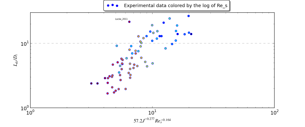
In the end, I used nls to explore the possible exponents of my fit. I also removed some outliers in my data that used a different experimental method. I settled on a fit that gave me decent Pr(>|t|) and residuals and which visually produce a decent fit. The last outlier is actually another experiment with a different setup, but one that I trust. So in a sense it's good that it shows up as an outlier as it hints at other parameters that need to be explored. Thank you gung, I accept your answer as I believe it guided me in the right direction.
> model = nls(L.D ~ C*I(J^(c1))*I(Re_s^(c2)), start=list(C=10,c1=-0.25,c2=-0.25),data=df)
> summary(model)
Formula: L.D ~ C * I(J^(c1)) * I(Re_s^(c2))
Parameters:
   Estimate Std. Error t value Pr(>|t|)
C  57.20389   26.40011   2.167   0.0337 *
c1 -0.27721    0.05901  -4.698 1.27e-05 ***
c2 -0.16424    0.04936  -3.327   0.0014 **
---
Signif. codes:  0 ‘***’ 0.001 ‘**’ 0.01 ‘*’ 0.05 ‘.’ 0.1 ‘ ’ 1
Residual standard error: 4 on 70 degrees of freedom
Number of iterations to convergence: 8
Achieved convergence tolerance: 2.91e-06


dcl ~ I(J^(-0.5))relationship is significant. Now you need to consider how Re could factor into this. Could it possibly modify the relationship between dcl and J? Than look at interactions. $\endgroup$