One-tailed t-test and confidence interval of difference in means

Question

Typical t-test checks if two sample means are significantly different from each other. Let's assume the following two sample sets:

x1 = [12.9, 10.2, 7.4, 7.0, 10.5, 11.9, 7.1, 9.9, 14.4, 11.3]
x2 = [10.2, 6.9, 10.9, 11.0, 10.1, 5.3, 7.5, 10.3, 9.2, 8.8]

Question: Is the mean of x1 significantly different from the mean of x2? (mu1 != mu2)

I can construct their 95% confidence interval of means:

stats.t.interval(1 - 0.05, len(x1) - 1, loc=np.mean(x1), scale=stats.sem(x1))
>>> (8.461873578892417, 12.058126421107586)

stats.t.interval(1 - 0.05, len(x2) - 1, loc=np.mean(x2), scale=stats.sem(x2))
>>> (7.663208497074507, 10.376791502925492)

There's an overlap between the two confidence intervals, and therefore the sample means are not significantly different. We can also formally test this using t-test assuming equal variance:

stats.ttest_ind(x1, x2, equal_var=False)
>>> Ttest_indResult(statistic=1.245268949149111, pvalue=0.23018336828903668)

Since the p-value is not smaller than 0.05, we cannot reject the null hypothesis, and conclude that sample means are not significantly different.

But what if I want to know if one group has higher means than the other?

Question: Is the mean of x1 significantly bigger than the mean of x2? (mu1 > mu2)

I've heard that there's a difference between two-tailed and one-tailed test, and I think my question is related to it. How can I tell if something is significantly BIGGER or LESS than the other? Not just something is significantly DIFFERENT from each other? How do I quantify that difference?

Answer 1

Welch one-tailed t test. A Welch (separate variances) 2-sample t test of $H_0: \mu_1 \le \mu_2$ against $H_a: \mu_1 > \mu_2$ in R gives the following result:

x1 = c(12.9, 10.2, 7.4, 7.0, 10.5, 11.9, 7.1, 9.9, 14.4, 11.3)
x2 = c(10.2, 6.9, 10.9, 11.0, 10.1, 5.3, 7.5, 10.3, 9.2, 8.8)

t.test(x1, x2, alte="gr")      # Note param 'alte="gr"` for right tailed test

        Welch Two Sample t-test

data:  x1 and x2
t = 1.2453, df = 16.74, p-value = 0.1151
alternative hypothesis: true difference in means is greater than 0
95 percent confidence interval:
 -0.4937982        Inf
sample estimates:
mean of x mean of y 
    10.26      9.02 

Testing with P-value: The sample mean $\bar X_1=10.62$ is not significantly larger than the sample mean $\bar X_2=9.02$ at the 5% level of significance because the P-value $0.115 > 0.05.$

For comparison: a two-tailed test of $H_0: \mu_1 = \mu_2$ against $H_a: \mu_1 \ne \mu_2$ would have a P-value about 0.23 (twice the P-value of the right-tailed test shown above). As you have seen: no significant difference.

Testing with critical value: Because the test statistic $T$ is approximately distributed according to Student's t distribution with 16.75 degrees of freedom, the critical value for a right tailed test at the 5% level is $c = 1.741,$ so that one would reject if $T > c = 1.741,$ but this is not the case. [Again for comparison, the critical value for a two-sided test would be $c = 2.112,$ with rejection for $|T| > 2.112,$ also not the case.]

qt(.95, 16.74)
[1] 1.741163
qt(.975, 16.74)
[1] 2.112315

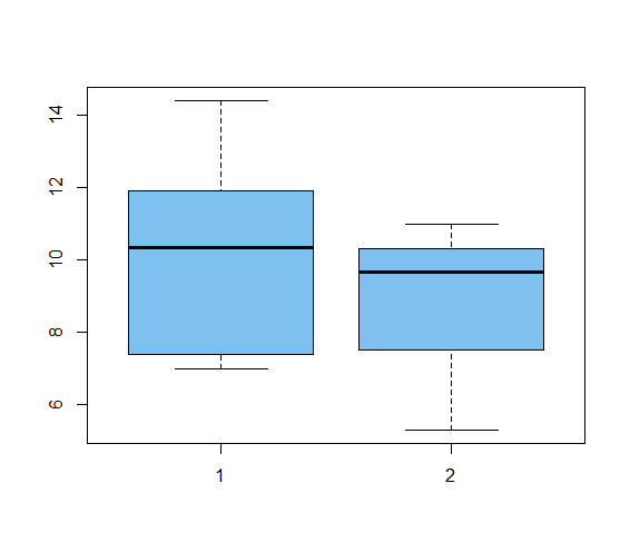
Visualization. Boxplots of the two samples, plotted sided-by-side on the same scale, illustrate the considerable overlap of values between the two samples.

boxplot(x1, x2, col="skyblue2")

For both the right-sided and the two-sided test, the null distribution is Student's t distribution with 16.74 degrees of freedom; its density function is shown in both graphs below. At left, the critical value $c = 1.741$ is located at the vertical dotted line; 5% of the area under the density curve lies to the right of that line. The solid blue vertical line shows the observed value $T = 1.25$ of the test statistic; the area under the density curve to the right of this line is the P-value. At right, the critical values $\pm 2.112$ are shown as dotted vertical lines, each cutting 2.5% of the area from a tail of the distribution. Taking into account that $T = -1.25$ would have be just as extreme (in the directions of the alternative) as $T = 1.25,$ the P-value gets doubled.

Notes: (1) Each sample separately is consistent with random sampling from a normal population. Samples are small, but we can see that there is no marked departure from normality that would interfere with the validity of a t test. (2) The sample variances are noticeably different, but not significantly different. Lacking advance information that the two populations have essentially the same variance, I followed standard practice and used the Welch t test, which does not assume equal population variances. (3) However, the P-value of of a right-tailed, 2-sample pooled t test is also about 0.11, so it wouldn't have found a significant difference either. (4) In the Welch test, R uses fractional degrees of freedom for the t distribution. Some software and almost all printed tables would use 16 or 17 degrees of freedom instead of 16.74; results for non-rejection would be unchanged.