Definition of the dirichlet process: what is the sequence of random variables

Question

Reference material by Dr. Teh

Definition

Given a measureable set S, a base probability distribution H and a positive real number $\alpha$, the Dirichlet process $DP(H, \alpha)$ is a stochastic process whose sample path is a probability distribution over $\Theta$, such that the following holds:

for any measureable finite partition of $\Theta$, denoted $\{A_i\}_{i=1}^r$, if $X \sim \text{DP}(H, \alpha)$, then

$$(X(A_1), ..., X(A_r)) \sim \text{Dirichlet}(\alpha H(A_1), ..., > \alpha H(A_r))$$

Questions

A stochastic process is a sequence of random variables indexed by some set $T$. A dirichlet process is a stochastic process, with the definitions above. My question is,

1) Given a sample path $\{X_1, X_2, \dots\}$, each $X_i$ (Not $X(A_i)$) is a probability vector of what size? How is the size determined?

2) I understand from definition that each are probability vectors drawn from a Dirichlet($\alpha H(A_1), \dots, \alpha H(A_r)$), but what are the partitions?

3) are there any relations between each $X_i$ to $X_{i+1}$? If so, how?

Edited questions to clear some ambiguities

Answer 1

The notes you reference have a splendid, clear, insightful discussion of this definition, its meaning, and its application--thank you for bringing them to our attention. Because the job of explanation has been so well done, all that is needed may be to clarify the specific points in your question. It looks like you lack only a definition of a "partition:"

A partition of a set $\mathcal{X}$ is a collection of its subsets $\mathcal{A}_i \subset \mathcal{X}$ for which (1) $\bigcup_{i} \mathcal{A_i}=\mathcal{X}$ and (2) $\mathcal{A}_i \cap \mathcal{A}_j = \emptyset$ whenever $i\ne j.$

The first condition says the subsets comprise all of $\mathcal X$ and the second says no two have any elements in common. Thus, every element of $X$ belongs to exactly one element of the partition.

Partitions may have any cardinality less than that of $\mathcal X$ itself. When the cardinality is finite, the partition is finite. In the notation of the question, $r$ is its cardinality--the number of distinct subsets in the partition.

Finally, $\Theta$ is endowed with a probability measure. Because the definition involves probabilities of the sets ("events") in the partition, they all need to be measurable subsets.

Thus:

1. Because $(X(\mathcal{A}_1), \ldots, X(\mathcal{A}_r))$ is a realization of a Dirichlet distribution, it must be a vector of $r$ non-negative components summing to unity.

2. The partitions are literally any possible partitions of $\Theta$ that meet the requirements of being finite and measurable.

3. $r$ is the cardinality of such an arbitrary partition.

4. The only relation between $X(\mathcal{A}_i)$ and $X(\mathcal{A}_j)$ is that required of any Dirichlet random variable: namely, these values are non-negative and they cannot sum to more than $1.$

Finally, don't think of a stochastic process in this context as a "sequence of random variables:" think of it as a randomly-chosen probability distribution on $\Theta.$ It can be approximated arbitrarily closely by binning $\Theta$ (that's what the partitioning does) into sufficiently small bins $\mathcal{A}_i$ and using a suitable Dirichlet distribution to realize the probability associated with each bin, written as $X(\mathcal{A}_i).$

---

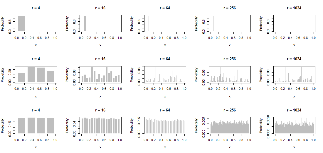
One way to visualize this is to draw a series of these approximations. In each row of the figure I use bar charts to plot the values of $X(\mathcal{A}_i), \ldots, X(\mathcal{A}_r)$ for the partition

$$\mathcal{A}_i = \left[\frac{i-1}{r}, \frac{i}{r}\right)$$

of the unit interval $\Theta = [0,1).$ The base measure $H$ is the uniform distribution on $\Theta.$ Each row depicts a single realization of the process $X.$ The rows have differing "inverse variance" parameters $\alpha,$ ranging from $1$ (top) to $100$ (middle) to $10000$ (bottom). In this downward progression you can see the sense in which the process $X$ tends to differ less and less from $H$ (whose density is constant) as $\alpha$ is increased. In the progressions from left to right, as $r$ is increased, you can see how more and more detail of each realization is brought out in the finer partitions. Think of a realization of the process as taking a limit as you move further out to the right.

It might be instructive to study the code that produced these realization, so here it is.

#
# Generate `n` realizations of a Dirichlet (p) random variable.
#
rdirichlet <- function(n, p) {
  v <- t(matrix(rgamma(n*length(p), p), ncol=n))
  v / rowSums(v)
}
#
# Coarsen a partition by combining successive sequences of `k` values.
#
gather <- function(x, k) {
  colMeans(matrix(x, nrow=k))
}
#
# Create realizations of a Dirchlet process.
#
alpha <- 1e0
n <- 2^10
x <- (1:n-1/2)/n

par(mfrow=c(3,5))
set.seed(17)
for (alpha in c(1, 1e2, 1e4)) {
  p <- n * rdirichlet(1, alpha * rep(1/n,n))
  for (i in rev(seq(0, 8, by=2))) {
    x.i <- gather(x, 2^i)
    p.i <- gather(p, 2^i) / length(x.i)
    plot(x.i, p.i, type="h", lwd=100/n*2^i, 
         xlim=0:1, ylim=c(0, max(p.i)),
         lend=1, col="Gray",
         main=paste("r =", n/2^i), xlab="x", ylab="Probability")
  }
}
par(mfrow=c(1,1))