Transformation to increase kurtosis and skewness of normal r.v

Question

I'm working on an algorithm that relies on the fact that observations $Y$s are normally distributed, and I would like to test the robustness of the algorithm to this assumption empirically.

To do this, I was looking for a sequence of transformations $T_1(), \dots, T_n()$ that would progressively disrupt the normality of $Y$. For example if the $Y$s are normal they have skewness $= 0$ and kurtosis $= 3$, and it would be nice to find a sequence of transformation that progressively increase both.

My idea was to simulate some normally approximately distributed data $Y$ and test the algorithm on that. Than test algorithm on each transformed dataset $T_1(Y), \dots, T_n(y)$, to see how much the output is changing.

Notice that I don't control the distribution of the simulated $Y$s, so I cannot simulate them using a distribution that generalizes the Normal (such as the Skewed Generalized Error Distribution).

Answer 1

This can be done using the sinh-arcsinh transformation from

Jones, M. C. and Pewsey A. (2009). Sinh-arcsinh distributions. Biometrika 96: 761–780.

The transformation is defined as

$$H(x;\epsilon,\delta)=\sinh[\delta\sinh^{-1}(x)-\epsilon], \tag{$\star$}$$

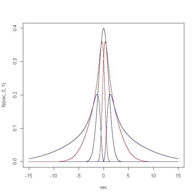
where $\epsilon \in{\mathbb R}$ and $\delta \in {\mathbb R}_+$. When this transformation is applied to the normal CDF $S(x;\epsilon,\delta)=\Phi[H(x;\epsilon,\delta)]$, it produces a unimodal distribution whose parameters $(\epsilon,\delta)$ control skewness and kurtosis, respectively (Jones and Pewsey, 2009), in the sense of van Zwet (1969). In addition, if $\epsilon=0$ and $\delta=1$, we obtain the original normal distribution. See the following R code.

fs = function(x,epsilon,delta) dnorm(sinh(delta*asinh(x)-epsilon))*delta*cosh(delta*asinh(x)-epsilon)/sqrt(1+x^2)

vec = seq(-15,15,0.001)

plot(vec,fs(vec,0,1),type="l")
points(vec,fs(vec,1,1),type="l",col="red")
points(vec,fs(vec,2,1),type="l",col="blue")
points(vec,fs(vec,-1,1),type="l",col="red")
points(vec,fs(vec,-2,1),type="l",col="blue")

vec = seq(-5,5,0.001)

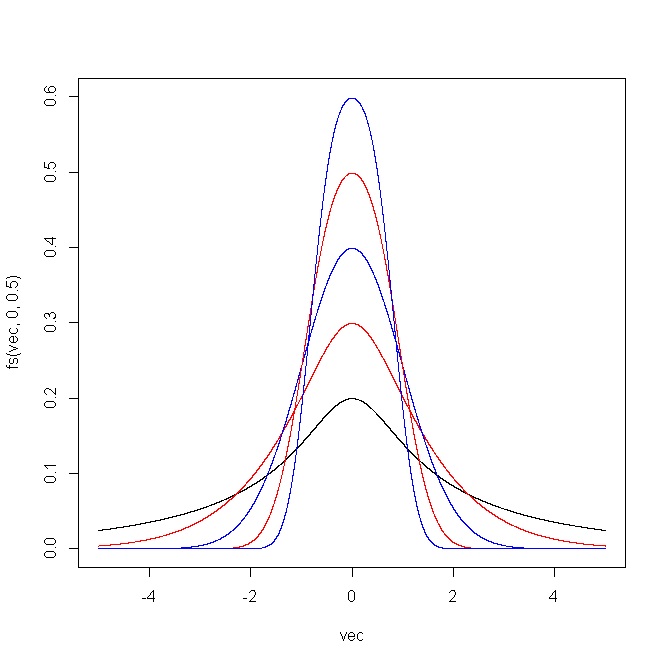
plot(vec,fs(vec,0,0.5),type="l",ylim=c(0,1))
points(vec,fs(vec,0,0.75),type="l",col="red")
points(vec,fs(vec,0,1),type="l",col="blue")
points(vec,fs(vec,0,1.25),type="l",col="red")
points(vec,fs(vec,0,1.5),type="l",col="blue")

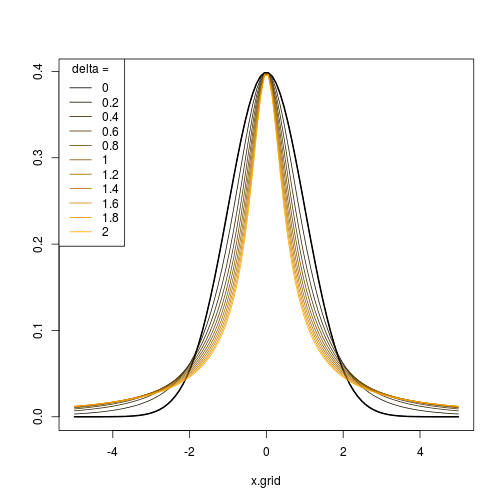
Therefore, by choosing an appropriate sequence of parameters $(\epsilon_n,\delta_n)$, you can generate a sequence of distributions/transformations with different levels of skewness and kurtosis and make them look as similar or as different to the normal distribution as you want.

The following plot shows the outcome produced by the R code. For (i) $\epsilon=(-2,-1,0,1,2)$ and $\delta=1$, and (ii) $\epsilon=0$ and $\delta=(0.5,0.75,1,1.25,1.5)$.

Simulation of this distribution is straightforward given that you just have to transform a normal sample using the inverse of $(\star)$.

$$H^{-1}(x;\epsilon,\delta)=\sinh[\delta^{-1}(\sinh^{-1}(x)+\epsilon)]$$

Answer 2

This can be done using Lambert W x F random variables / distributions. A Lambert W x F random variable (RV) is a non-linearly transformed (RV) X with distribution F.

For F being the Normal distribution and $\alpha = 1$, they reduce to Tukey's h distribution. The nice property of Lambert W x F distributions is that you can also go back from non-normal to Normal again; i.e., you can estimate parameters and Gaussianize() your data.

They are implemented in the

Lambert W x F transformations come in 3 flavors:

• skewed (type = 's') with skewness parameter $\gamma \in R$
• heavy-tailed (type = 'h') with tail parameter $\delta \geq 0$ (and optional $\alpha$)
• skewed and heavy tailed (type = 'hh') with left/right tail parameter $\delta_l, \delta_r \geq 0$

See References on skewed and heavy-tail(s) (Disclaimer: I am the author.)

In R you can simulate, estimate, plot, etc. several Lambert W x F distributionswith the LambertW package.

library(LambertW)
library(RColorBrewer)
# several heavy-tail parameters
delta.v <- seq(0, 2, length = 11)
x.grid <- seq(-5, 5, length = 100)
col.v <- colorRampPalette(c("black", "orange"))(length(delta.v))

plot(x.grid, dnorm(x.grid), lwd = 2, type = "l", col = col.v[1],
     ylab = "")
for (ii in seq_along(delta.v)) {
  lines(x.grid, dLambertW(x.grid, "normal", 
                          theta = list(delta = delta.v[ii], beta = c(0, 1))),
        col = col.v[ii])
}
legend("topleft", paste(delta.v), col = col.v, lty = 1,
       title = "delta = ")

It works similarly for a sequence of $\gamma$ to add skewness. And if you want to add skewness and heavy-tails then generate a sequence of $\delta_l$ and $\delta_r$.

Answer 3

One such sequence is exponentiation to various degrees. E.g.

library(moments)
x <- rnorm(1000) #Normal data
x2 <- 2^x #One transformation
x3 <- 2^{x^2} #A stronger transformation
test <- cbind(x, x2, x3) 
apply(test, 2, skewness) #Skewness for the three distributions
apply(test, 2, kurtosis) #Kurtosis for the three distributions

You could use $x^{1.1}, x^{1.2} \dots x^2$ to get intermediate degrees of transformation.

Answer 4

Same answer as @user10525 but in python

import numpy as np
from scipy.stats import norm
def sinh_archsinh_transformation(x,epsilon,delta):
    return norm.pdf(np.sinh(delta*np.arcsinh(x)-epsilon))*delta*np.cosh(delta*np.arcsinh(x)-epsilon)/np.sqrt(1+np.power(x,2))


vec = np.arange(start=-15,stop=15+0.001,step=0.001)

import matplotlib.pyplot as plt
plt.plot(vec,sinh_archsinh_transformation(vec,0,1))
plt.plot(vec,sinh_archsinh_transformation(vec,1,1),color='red')
plt.plot(vec,sinh_archsinh_transformation(vec,2,1),color='blue')
plt.plot(vec,sinh_archsinh_transformation(vec,-1,1),color='red')
plt.plot(vec,sinh_archsinh_transformation(vec,-2,1),color='blue')

[