First a warning... the Bootstrap (as with most statistical methods) is unlikely to be reliable with such a small sample size. I would exercise caution if $n=6$ is a standard sample size in your case.
Lets simulate some data
set.seed(42)
n <- 30 #Sample size
x <- round(runif(n, 0, 100))
Lets refer to your index as $\theta$ and the estimator you provide for it as $\hat\theta$, which can be computed as follows.
theta_hat <- var(x)/mean(x)^2 - 1/mean(x)
For this simulated data, I get $\hat\theta = 0.2104$ and (by assuming $\hat\theta$ is a consistent estimator and cranking $n$ wayyyy up) we have roughly $\theta = 0.32$.
Obtain the Bootstrap distribution
The Bootstrap algorithm is fairly straightforward to code up on your own.
B <- 10000 #number of bootstrap resamples
theta_boot <- rep(NA, B)
for(i in 1:B){
  #Select a bootstrap sample
  xnew <- sample(x, length(x), replace=TRUE)
  #Estimate index
  theta_boot[i] <- var(xnew)/mean(xnew)^2 - 1/mean(xnew)
}

#Plot bootstrap distribution
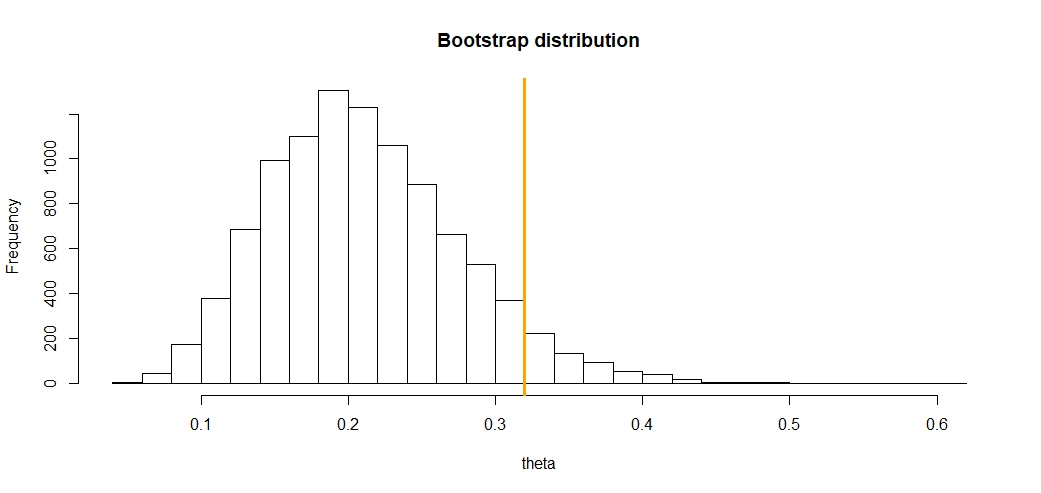
hist(theta_boot, breaks=30, xlab='theta', main='Bootstrap distribution')
abline(v=0.32, lwd=2, col='orange')
The resulting distribution looks like this, where the vertical line represents the "true" value of the index $\theta$.

Confidence intervals using the (percentile) Bootstrap
At this point, getting a confidence interval is very straightforward. Suppose you want a $95\%$ CI (i.e. $\alpha = 0.05$). You are looking for the points $L$ and $U$ such that $2.5\%$ of the Bootstrap samples are below $L$ and above $U$.
Mathematically, this is equivalent to setting
$$L = \hat F^{-1}(\alpha/2) \quad\quad\quad U = \hat F^{-1}(1-\alpha/2),$$
where $\hat F$ is the "Bootstrap CDF". In R, this can be done simply by typing
alpha <- 0.05
quantile(theta_boot, c(alpha/2, 1-alpha/2))
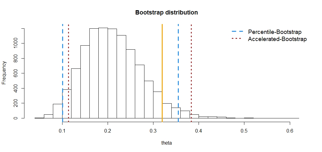
For this data, we get a $95\%$ CI of $(0.101, 0.355)$.
The Accelerated Bootstrap
Although the method of the previous section is a straightforward and natural way to obtain endpoints for a confidence interval, there are several alternatives which have been shown to perform better in a variety of settings. The Accelerated Bootstrap is one such method.
The endpoints to the CI in this approach are found by considering the function
$$g(u) = \hat F^{-1}\left(\Phi\left(z_0 + \frac{z_0 + z_u}{1-a(z_0+z_u)}\right) \right)$$
and setting $L = g(\alpha/2)$ and $U=g(1-\alpha/2)$. There are a lot of new terms in this function which I will now describe.
- $\Phi(z)$ represents the standard normal CDF.
- $z_0 = \Phi^{-1}(\hat F(\hat\theta)).$
- $z_u = \Phi^{-1}(u).$
- $a$ is an "acceleration constant".
Estimation of the acceleration constant is the last remaining "challenge" and will be discussed in the next section. For now, let's fix the value $a=0.046$. The accelerate Bootstrap CI can now be computed in R as follows.
#Desired quantiles
u <- c(alpha/2, 1-alpha/2)

#Compute constants
z0 <- qnorm(mean(theta_boot <= theta_hat))
zu <- qnorm(u)
a <- 0.046

#Adjusted quantiles
u_adjusted <- pnorm(z0 + (z0+zu)/(1-a*(z0+zu)))

#Accelerated Bootstrap CI
quantile(theta_boot, u_adjusted)
This gives a new $95\%$ CI of $(0.114, 0.383)$, which has effectively "shifted" the CI bounds in the direction of the true value for $\theta$. (Side note: when $a=0$, the accelerated Bootstrap is known as the bias correction Bootstrap).
The following figure shows the Bootstrap distribution again, with vertical lines representing the Confidence intervals for each case.

Estimating the acceleration constant
The acceleration constant can (in some cases) be calculated theoretically from the data by assuming a particular distribution for the data. Otherwise, a non-parametric approach can be used.
Efron (1987) shows that for univariate sampling distributions, the acceleration constant is reasonably well approximated by
$$\hat a = \frac{1}{6}\frac{\sum_{i=1}^n I_i^3}{\left(\sum_{i=1}^nI_i^2\right)^{3/2}}$$
where $I_i$ denotes the influence of point $x_i$ on the estimation of $\theta$. Efron proposes approximating $I_i$ using the infinitesimal jackknife, but others have demonstrated that the finite-sample Jackknife is often sufficient. Thus, each $I_i$ can be approximated by
$$I_i = (n-1)[\hat\theta - \hat\theta_{-i}]$$
where $\hat\theta_{-i}$ represents an estimate of $\theta$ (your index) after removing the $i^{th}$ data point.
I <- rep(NA, n)
for(i in 1:n){
   #Remove ith data point
   xnew <- x[-i]
   #Estimate theta
   theta_jack <- var(xnew)/mean(xnew)^2 - 1/mean(xnew)
   I[i] <- (n-1)*(theta_hat - theta_jack)
}
#Estimate a
a_hat <- (sum(I^3)/sum(I^2)^1.5)/6
This leads to the acceleration constant estimate of $\hat a = 0.046$ that was used in the previous section.
Edit (May 2024)
For interested parties, there is an R implementation of the accelerated bootstrap (as presented here) in this R package (on github). The package can be installed using the devtools package with the command devtools::install_github("knrumsey/quack"). The relevant functions include est_accel() and boot_accel().

