8
$\begingroup$

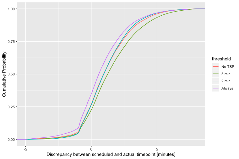
I am trying to determine if there is a statistically meaningful distinction between the cumulative probability density curves shown in the figure below.

Cumulative Probability Distribution

It's simple enough to do a $t$-test on the means of these distributions. But I am also looking to see if the treatment has an effect at more extreme values of the density distribution. For instance, if the means are the same but the 85th percentiles are different, that is something I would be interested in.

The 95% confidence interval of the mean is roughly $\bar{x} \pm 1.95 \sigma_x$. But it doesn't feel right to use the same variance at every level of the CDF, especially when the empirical distribution is largely non-normal.

$\endgroup$
4
  • $\begingroup$ I’ve done a bootstrap confidence interval of the differences at each quantile, say 0.01 to 0.99 in increments of 0.01. There may be functions to do this, though it’s pretty easy in R with the ecdf function. You can argue against correcting for multiple hypothesis tests by doing something like first KS testing and not testing quantiles unless KS rejects. I would expect there to be other ways, too, such as smoothing your results to smooth away spurious rejections. I find your language of “statistically meaningful” to be interesting, though, and worth discussing. What do you mean by that? $\endgroup$
    – Dave
    Commented Dec 19, 2019 at 23:45
  • $\begingroup$ I guess I wanted to avoid saying "statistically significant" but I suppose that's what I meant. $\endgroup$ Commented Dec 19, 2019 at 23:46
  • $\begingroup$ I didn’t realize that there were four distributions. Unless you want to do pair-wise comparisons, bootstrapping the differences will not work. $\endgroup$
    – Dave
    Commented Dec 19, 2019 at 23:48
  • $\begingroup$ However, it seems like you want CIs on each CDF, so I do think you can bootstrap each distribution (separately) and calculate a confidence interval at every quantile of interest for each distribution. $\endgroup$
    – Dave
    Commented Dec 20, 2019 at 0:03

3 Answers 3

5
$\begingroup$

You can do something like this with simultaneous-quantile regression with a set dummies corresponding to the 4 groups. This allows you to test and construct confidence intervals comparing coefficients describing different quantiles that you care about.

Here's a toy example where we cannot reject the joint null that the 25th, 50th, and 75th quartile of car prices are all equal in all 4 MPG groups (the p-value is 0.374):

. sysuse auto, clear
(1978 Automobile Data)

. xtile mpg_quartile = mpg, nq(4)

. distplot price, over(mpg_quartile) legend(rows(1)) ylab(.25 .5 .75, angle(0) grid) xlab(#10, grid) ///
> plotregion(fcolor(white) lcolor(white)) graphregion(fcolor(white) lcolor(white))

. 
. sqreg price i.mpg_quart, quantile(.25 .5 .75) reps(500)
(fitting base model)

Bootstrap replications (500)
----+--- 1 ---+--- 2 ---+--- 3 ---+--- 4 ---+--- 5 
..................................................    50
..................................................   100
..................................................   150
..................................................   200
..................................................   250
..................................................   300
..................................................   350
..................................................   400
..................................................   450
..................................................   500

Simultaneous quantile regression                    Number of obs =         74
  bootstrap(500) SEs                                .25 Pseudo R2 =     0.0909
                                                    .50 Pseudo R2 =     0.1228
                                                    .75 Pseudo R2 =     0.2639

------------------------------------------------------------------------------
             |              Bootstrap
       price |      Coef.   Std. Err.      t    P>|t|     [95% Conf. Interval]
-------------+----------------------------------------------------------------
q25          |
mpg_quartile |
          2  |      -1297   528.3106    -2.45   0.017    -2350.682   -243.3178
          3  |      -1192   447.9346    -2.66   0.010    -2085.377   -298.6225
          4  |      -1484   458.6527    -3.24   0.002    -2398.754   -569.2459
             |
       _cons |       5379   414.9198    12.96   0.000     4551.468    6206.532
-------------+----------------------------------------------------------------
q50          |
mpg_quartile |
          2  |      -1442   1253.755    -1.15   0.254    -3942.535    1058.535
          3  |      -1086   1414.436    -0.77   0.445    -3907.004    1735.004
          4  |      -1776   1232.862    -1.44   0.154    -4234.867    682.8667
             |
       _cons |       6165   1221.461     5.05   0.000     3728.873    8601.127
-------------+----------------------------------------------------------------
q75          |
mpg_quartile |
          2  |      -6213   1591.987    -3.90   0.000    -9388.118   -3037.882
          3  |      -4535   1847.591    -2.45   0.017    -8219.904   -850.0963
          4  |      -6796   1592.095    -4.27   0.000    -9971.334   -3620.666
             |
       _cons |      11385   1556.486     7.31   0.000     8280.686    14489.31
------------------------------------------------------------------------------

. test ///
> ([q25]2.mpg_quart=[q25]3.mpg_quart=[q25]4.mpg_quart) ///
> ([q50]2.mpg_quart=[q50]3.mpg_quart=[q50]4.mpg_quart) ///
> ([q75]2.mpg_quart=[q75]3.mpg_quart=[q75]4.mpg_quart)

 ( 1)  [q25]2.mpg_quartile - [q25]3.mpg_quartile = 0
 ( 2)  [q25]2.mpg_quartile - [q25]4.mpg_quartile = 0
 ( 3)  [q50]2.mpg_quartile - [q50]3.mpg_quartile = 0
 ( 4)  [q50]2.mpg_quartile - [q50]4.mpg_quartile = 0
 ( 5)  [q75]2.mpg_quartile - [q75]3.mpg_quartile = 0
 ( 6)  [q75]2.mpg_quartile - [q75]4.mpg_quartile = 0

       F(  6,    70) =    1.10
            Prob > F =    0.3740

The ECDF looks like this:
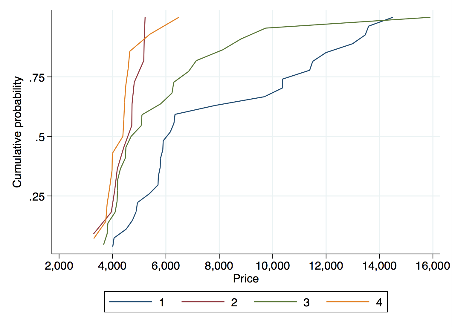
enter image description here

Though there seem to be large differences between group 1 and groups 2-4 for the 3 quantiles in the graph. However, this is not a lot of data, so the failure to reject with the formal test is perhaps not that surprising because of the "micronumerosity".

Interestingly, the Kruskal-Wallis test of the hypothesis that 4 groups are from the same population rejects:

. kwallis price , by(mpg_quartile)

Kruskal-Wallis equality-of-populations rank test

  +---------------------------+
  | mpg_qu~e | Obs | Rank Sum |
  |----------+-----+----------|
  |        1 |  27 |  1397.00 |
  |        2 |  11 |   286.00 |
  |        3 |  22 |   798.00 |
  |        4 |  14 |   294.00 |
  +---------------------------+

chi-squared =    23.297 with 3 d.f.
probability =     0.0001

chi-squared with ties =    23.297 with 3 d.f.
probability =     0.0001
$\endgroup$
4
  • $\begingroup$ @gregmacfarlane Did this help? $\endgroup$
    – dimitriy
    Commented Jan 6, 2020 at 19:36
  • $\begingroup$ It did help! But I had to put it aside for about a year. But this month I picked it up again, and I think that this is what I'm going with. $\endgroup$ Commented May 17, 2021 at 19:22
  • $\begingroup$ I ended up using the quantreg package for R. Worked like a charm. $\endgroup$ Commented May 24, 2021 at 16:47
  • $\begingroup$ Glad to hear that! $\endgroup$
    – dimitriy
    Commented May 24, 2021 at 16:47
6
$\begingroup$

Assuming that your curves represent the empirical CDFs obtained from data, the usual way to test for a difference between more than two groups would be some kind of multi-sample non-parametric test akin to the Kolmogorov-Smirnov test, or a rank-based ANOVA test like the multi-sample Kruskal-Wallis test. There are a number of papers in the statistical literature looking at multi-sample non-parameetric tests of this kind (see e.g., Kiefer 1959, Birnbaum and Hall 1960, Conover 1965, Sen 1973 for early literature). If you reduce down to a pairwise comparison of interest, you can of course use the traditional two-sample tests.

There is an R package called ksamples that implements the multi-sample Kruskal-Wallis test and some other multi-sample non-parametric tests. I am not aware of a package that does the multi-sample KS test, but others may be able to point you to additional resources.

$\endgroup$
2
  • $\begingroup$ Something like KS will be sensitive to more than just differences in mean. However, would any of these get at particular quantities where there are differences? $\endgroup$
    – Dave
    Commented Dec 20, 2019 at 1:18
  • 1
    $\begingroup$ These tests look for differences in the entire CDF, not just differences in means. If I understand the question correctly, this appears to be what the OP is interested in. $\endgroup$
    – Ben
    Commented Dec 20, 2019 at 2:18
3
$\begingroup$

For comparing 2 distributions at a time ("pairwise"), it's possible to find all the ranges of values for which the CDFs are statistically significantly different, while controlling the familywise error rate (FWER) at your desired level. This (new) approach is described in detail in this 2018 Journal of Econometrics paper, as well as in this 2019 Stata Journal article. R and Stata code (and open drafts of articles, and replication files) are at https://faculty.missouri.edu/~kaplandm. Both articles include examples with real data. Everything is fully nonparametric, and the "strong control" of FWER is exact even in small samples.

$\endgroup$

Your Answer

By clicking “Post Your Answer”, you agree to our terms of service and acknowledge you have read our privacy policy.

Not the answer you're looking for? Browse other questions tagged or ask your own question.