Difference between linear model and linear mixed model

Question

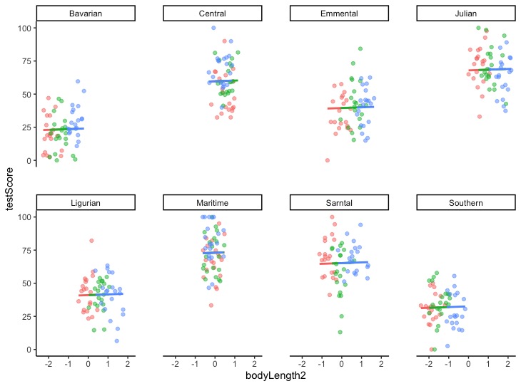
I am confused about the difference between linear model (LM) and linear mixed model (LMM). I use an example from Introduction to linear mixed models. Grateful if you can explain the subtle differences between 2 models by using the example below.

The LM I use is:

mountain.lm <- lm(testScore ~ bodyLength2 + mountainRange, data = dragons)
summary(mountain.lm)

The summary shows:

Coefficients:
                      Estimate Std. Error t value Pr(>|t|)    
(Intercept)            23.3818     2.5792   9.065  < 2e-16 ***
bodyLength2             0.2055     1.2927   0.159  0.87379    
mountainRangeCentral   36.5828     3.5993  10.164  < 2e-16 ***
mountainRangeEmmental  16.2092     3.6966   4.385 1.43e-05 ***
mountainRangeJulian    45.1147     4.1901  10.767  < 2e-16 ***
mountainRangeLigurian  17.7478     3.6736   4.831 1.84e-06 ***
mountainRangeMaritime  49.8813     3.1392  15.890  < 2e-16 ***
mountainRangeSarntal   41.9784     3.1972  13.130  < 2e-16 ***
mountainRangeSouthern   8.5196     2.7313   3.119  0.00192 ** 

The ggplot by:

facet_wrap(~mountainRange, nrow=2)

---

The LMM I use is:

mixed.lmer <- lmer(testScore ~ bodyLength2 + (1|mountainRange), data = dragons)
summary(mixed.lmer)

The summary shows:

Random effects:
 Groups        Name        Variance Std.Dev.
 mountainRange (Intercept) 339.7    18.43   
 Residual                  223.8    14.96   
Number of obs: 480, groups:  mountainRange, 8

Fixed effects:
            Estimate Std. Error t value
(Intercept)  50.3860     6.5517   7.690
bodyLength2   0.5377     1.2750   0.422

The ggplot:

The 2 plots look similar but I notice their slopes of bodylength2 are different: 0.2055 in LM, while 0.5377 in LMM. My understanding is if I want to explore the relationship between bodylength2 and testScore, I shall set mountainRange as a random effect, which means I shall use LMM. However, I can also explore the same relationship by using LM: the slopes are the same across mountainRange, which means the effect of mountainRange has been controlled. I am wondering what's the advantage of using LMM here. It would be better if you can explain in a simply mathematical way. Thanks!

Answer 1

You are correct that you can use either OLS (lm) to analyze nested data such as the toy data you have here. In doing so, you included dummy variables for each of the mountainRange groups except for a reference group. This is called a no-pooling model because no information is shared between the various mountainRange groups. Each gets its own intercept, directly estimated as a predictor in lm.

The non-dummy group predictors in the no-pooling lm model represent the average within-group association between bodyLength2 and testScore. Why? Because by entering the dummy for the group, it sucks up all between-group variation in predictors, leaving only within-group variation to explain within-group variation in the outcome.

In contrast, the mixed model allows the mountainRanges to share a common intercept but posits that they come from a larger population of mountainRanges. This is sometimes referred to as partial-pooling because information is shared among the groups. The mixed model separates variance in the outcome into variance that is within groups and also variance that is between groups. However, it does not separate the variance of predictors into within- and between-group portions. The analyst must do that themselves. Take your bodyLength variable. It varies within groups and also between groups. In order to separate the within- from between-group parts of the predictor, you can add the group mean of bodyLength as a predictor in your model.

First calculate the group mean for bodyLength:

require(dplyr)
dragons <- dragons %>% group_by(mountainRange) %>% mutate(mn_body2 = mean(bodyLength2)) %>% ungroup() 

Then add it to a new lmer model:

mixed.lmer2 <- lmer(testScore ~ bodyLength2 + mn_body2 + (1|mountainRange), dragons)
summary(mixed.lmer2)

Random effects:
 Groups        Name        Variance Std.Dev.
 mountainRange (Intercept) 260.3    16.13   
 Residual                  223.8    14.96   
Number of obs: 480, groups:  mountainRange, 8

Fixed effects:
            Estimate Std. Error t value
(Intercept)  50.3860     5.7449   8.771
bodyLength2   0.2055     1.2927   0.159
mn_body2     12.2016     6.8978   1.769

You will notice that the coefficient for bodyLength2 is exactly equivalent to the no-pooling estimate of this coefficient from lm. By including the mn_body2 in the mixed model, we have removed the between-group portion of variance in bodyLength2, so it is now providing a purely within-group estimate of the association between bodyLength2 and testScore.

The advantage of the mixed model is that it allows you examine both within- and between-group information as it relates to predictors and your outcome whereas the lm model with group dummies can only give you within-group information.

See also: Are covariates in a mixed model estimated between-group, within-group, or somewhere in-between? And why?