Does p-value ever depend on the alternative?

Question

Our tag definition of the $p$-value says

In frequentist hypothesis testing, the $p$-value is the probability of a result as extreme (or more) than the observed result, under the assumption that the null hypothesis is true.

I guess this is how Fisher thought about it, and I am comfortable with it. However, I think I have seen $p$-value being calculated differently in one-sided hypothesis testing. Outcomes that are not in the direction of the alternative do not get considered extreme.

E.g. assume $X\sim N(\mu,\sigma^2)$ and test $$ H_0\colon\mu=0 $$ against $$ H_1\colon\mu\neq 0. $$ Using the empirical mean $\bar x$ as an estimator of $\mu$, the $p$-value is calculated exactly as defined above. If $\bar x$ is far from zero (to either side) in terms of the estimated standard deviation $\hat\sigma$, the $p$-value is low.

Now consider $$ H_1'\colon\mu>0, $$ I have seen $p$-value calculated as $$ \text{p-value}=1-\text{CDF}(t) $$ where $t:=\frac{\bar x}{\hat\sigma/\sqrt{n}}$ is the $t$-statistic and $\text{CDF}$ is the cumulative density function of $t$ under $H_0$. Then $p$-value is high when $\bar x$ is far to the left of zero, contrary to the case above. $\bar x$ being far to the left of zero is extreme in the perspective of $H_0$, but in an uninteresting direction from the perspective of $H_1'$.

Questions: Does the p-value actually depend on the alternative hypothesis? Or is $\text{p-value}=1-\text{CDF}(\bar x)$ nonsense? Or are there alternative definitions depending on whether one uses Fisher's perspective, Neyman-Pearson perspecitve or some mixture of the two?

Edit 1: The definition of the term extreme appears to be crucial. One way of defining extreme is w.r.t. the probability density of the null distribution at the observed result; the lower the density, the more extreme the result. I guess this is how Fisher would have thought (there was a discussion about it somewhere on CV and/or in some paper, I think; I need some time to find it). Another way is to refer to the alternative hypothesis and pick the "interesting" extremes among all, though in my understanding (which could of course be wrong) this would be in conflict with the CV's definition cited above.

Edit 2: Thanks to Alexis for a good catch: if we are to choose an alternative $H_1'\colon \mu>0$, then the null becomes $H_0\colon \mu \leq 0$, and so values of $\mu$ to the left of zero are no longer extreme under the null. So it appears my example was faulty. Let us switch to another example which hopefully illustrates the main point better. In a multiple linear regression model, consider an overall $F$-test $H_0\colon \beta=0$. The alternative is not one-sided, but the distribution of the test statistic under the alternative is to the right of the null distribution, hence only the right tail is "interesting". The questions remain the same.

Edit 3: Here is a quote from Rob J. Hyndman's blog that, among other things, led to my questions:

Another thing I dislike about statistical tests is the alternative hypothesis. This was not originally part of hypothesis testing as proposed by Fisher. It was introduced by Neyman and Pearson. Frankly, the alternative hypothesis is unnecessary. It is not used in the computation of p-values or for determining statistical significance. The only practical use for the alternative hypothesis that I can see is in determining the power of a test.

(Emphasis is mine.)

---

A related question: "Defining extremeness of test statistic and defining $p$-value for a two-sided test".

Answer 1

The alternative hypothesis affects the test through the evidentiary ordering

The p-value of a classical hypothesis test depends on the alternative hypothesis only through the evidentiary ordering constructed for the test, which is what tells you what constitutes an "extreme" observation. Any hypothesis test involves specification of an evidentiary ordering which is a total preorder on the set of all possible outcomes of the observable data. This evidentiary ordering specifies which outcomes are more conducive to the null or alternative hypotheses respectively. Often this ordering is implicit on having defined a "test statistic" for the test, but the only role of the test statistic is to represent this ordering.

---

Hypothesis testing via an evidentiary ordering: Suppose we want to create a hypothesis test for an unknown parameter $\theta \in \Theta$ using an observable random vector $\mathbf{X} \in \mathscr{X}$ with a distribution that depends on this parameter. For any stipulated null space $\Theta_0$ and alternative space $\Theta_A$ (and any particular logic for how the test works) we contruct a total preorder $\succeq$ on the outcome space $\mathscr{X}$. The interpretation of the total preorder is:

$$\mathbf{x} \succeq \mathbf{x}' \quad \quad \iff \quad \quad \mathbf{x} \text{ is at least as conducive to } H_A \text{ as } \mathbf{x}'.$$

For brevity, we sometimes say that $\mathbf{x} \succeq \mathbf{x}'$ means that $\mathbf{x}$ is at least as "extreme" as $\mathbf{x}'$. This is a common shorthand, which is okay if you remember that "extreme" means "conducive to the alternative hypothesis" in this context. In practice, the evidentiary ordering for the sample space is often set implicitly by constructing a test statistic and having an ordering for the test statistic.$^\dagger$ This is essentially just the same thing, but removed one-level of abstraction away from the sample space in order to concentrate entirely on the ordering.

You should bear in mind that the situation is complicated slightly by the fact that the "test statistic" and "evidentiary ordering" may both be dependent on the parameter in the analysis. In fact, the "test statistic" is typically not a statistic, but often instead a pivotal quantity that depends on the parameter value in the hypothesis. In this case the evidentiary ordering will also be implicitly dependent on the parameter. (In the case of a test with a simple null hypothesis this doesn't matter, because the test always conditions on this single value. In the case of a test with a composite hypothesis it might matter, because the ordering now changes over the null space.) Taking this dependence as implicit for now, once we have set the evidentiary ordering for the test, the p-value function is then defined as:

$$p(\mathbf{x}) \equiv \sup_{\theta \in \Theta_0} \mathbb{P}(\mathbf{X} \succeq \mathbf{x} | \theta) \quad \quad \quad \text{for all } \mathbf{x} \in \mathscr{X}.$$

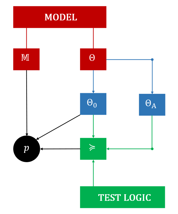
If we denote the probabilistic model by $\mathbb{M} \equiv \{ \mathbb{P}(\cdot | \theta) | \theta \in \Theta \}$ then we can write the p-value function as a function $p = f(\mathbb{M}, \Theta_0, \succeq)$. We can see that the p-value function is fully determined by the model $\mathbb{M}$, the null space $\Theta_0$ and the evidentiary ordering $\succeq$. Observe that the alternative hypothesis only affects this function through its contribution to the evidentiary ordering.

The structure of a classical hypothesis test is shown in the diagram below. This diagram illustrates the elements of the test that lead to the p-value function, which ultimately defines the test. As can be seen in the diagram, the alternative hypothesis has a limited role; combined with the logic of the test it affects the evidentiary ordering for the test, which then flows into determination of the p-value function.

One final thing that is worth noting in relation to this issue is that a classical hypothesis test is essentially an inductive analogue to the deductive proof by contradiction (see related answers here and here). In a proof by contradiction we begin with a null hypothesis, show that this leads logically to a contradiction, and therefore reject the initial premise that the null is true (with certainty). In a classical hypothesis test, we begin with a null hypothesis, show that this leads to a highly implausible result in favour of the alternative (so not quite a deductive contradiction, but close), and therefore reject the initial premise that the null is true (but with some uncertainty). The p-value in this test is the probability of a result at least as conducive to the alternative hypothesis, assuming the null is true. If this is low then it means that something very implausible happened (under the assumption that the null is true) which gives the "contradiction" in the "inductive proof by contradiction". Just as with a proof by contradiction, this procedure is asymmetric in the hypotheses and it is only necessary to look at things conditional on the null hypothesis. The alternative hypothesis contributes only to the extent that it helps us understand what is a more implausible result under the null hypothesis (i.e., through the evidentiary ordering) which allows us to inductively measure the "implausibility" that is analogous to a contradiction.

---

$^\dagger$ Often the evidentiary ordering is set implicitly using a test statistic $T: \mathscr{X} \rightarrow \mathbb{R}$ and then using the ordering defined by the correspondence $\mathbf{x}_0 \succeq \mathbf{x}_1 \iff T(\mathbf{x}_0) \geqslant T(\mathbf{x}_1)$. In this case the p-value reduces to $p(\mathbf{x}) = \sup_{\theta \in \Theta_0} \mathbb{P}(T(\mathbf{X}) \geqslant T(\mathbf{x}) | \theta)$.

Answer 2

The test statistic ($t$ in your example) and all calculations to reach that point depend only on the null hypothesis $H_0$ and nothing else.

The p-value is affected by the alternative hypothesis $H_1$ as the $H_1$ identifies which values are considered as "extreme" values and the p-value calculates the proximity of the final result (your $t$) to those values.

For instance, in your example of $H_0$ vs $H_1'$ you would reject $H_0$ only if $t>T_\alpha$ and for the example $H_0$ vs $H_1$ you would reject $H_0$ only if $t>T_{\alpha/2}$ or $t<-T_{\alpha/2}$.

Thus the p-value of $H_0$ vs $H_1$ would be the probability of the union of two sets whereas the $H_0$ vs $H_1'$ would be the probability of one set where the cut-off point is higher on the x-axis compared to the previous case.

EDIT: In response to what you mentioned about Fisher, I believe you are referring to the famous lady testing test. Which indeed doesn't have a strictly speaking alternative hypothesis but it is slightly different compared to the hypothesis tests that we usually conduct.

In this example, he only defined the null hypothesis $H_0$: She has no ability to distinguish the tea and he used the combination formula to measure the probability of all possible outcomes given that $H_0$ is true which is essentially the p-value of each data point.

The main difference/trick here that you might be looking for is that in Fisher's eyes, it would only take one incorrect guess to make her a liar and thus he wanted to identify the smallest amount of cups that he needs to give her to taste. In a sense, one might say that he tested the $H_1:$At least one incorrect guess and he looked for the smallest possible sample size for some pre-defined parameters.

This is a slightly different case to the way we usually conduct statistical hypothesis tests as we take sample from a population and we usually "allow" some non-$H_0$ cases. I guess the final answer to your question is that we want an $H_1$ or at least a "loose-definition" of it in order to define what are the "extreme-departures" from the $H_0$ (Even if you are Fisher and you hide it well enough).

Really good question by the way :)

Answer 3

Here's how I see it. Generally, the p-value is the probability, under the null hypothesis, to observe a result that is as far or farther away from what would be "typical" under the null hypothesis.

This is informal and imprecise, and in fact decisions need to be made in order to make this precise.

What needs to be chosen is a test statistic, and "far or farther away" needs to be defined. One way of doing this is to specify an alternative, and to ask, how does a test need to look like in order to achieve optimal power under the alternative while respecting the nominal level under the null hypothesis? This is Neyman and Pearson's approach to construct tests. Given the test statistic and the "direction" of the alternative (one-sided or two-sided, although in principle more complex "direction definitions" are conceivable), the p-value is computed using the null hypothesis and not the alternative. However the alternative has its impact through the determination of test statistic and direction.

Alternatively (!) one can choose the test statistic without specifying an alternative based on a (usually heuristic) idea of how to measure "closeness" to the null hypothesis (e.g., Kolmogorov-Smirnov or $\chi^2$-distance from the hypothesised distribution), preferably in such a way that the distribution of the test statistic under the null can be specified. This also requires a "direction", but this seems often trivial (e.g., large KS-distance => evidence against the null). In this case one could argue that there is no alternative and therefore no impact of the alternative on the p-value. One could however also say that a test constructed in this way implicitly defines an alternative, namely "all distributions that tend to generate test statistic values in the rejection direction".

As an example, consider the KS-test for normality. Though counter-intuitive at first sight, it is conceivable to reject normality in case of a too small KS-distance, which makes sense in an application in which it is suspected that researchers faked data in order to make them look "perfectly normal". The alternative to i.i.d. normality is then implicitly the family of distributions that tend to generate samples that look more normal than i.i.d. normal samples, for example because observations are dependent in such a way that a small KS-distance is enforced.

The p-value is then different from the standard KS-test. Not sure whether you'd say "this is because it depends on the alternative" because all these choices could be made without explicitly specifying an alternative, however it can for sure be related to the concept of an "implicit alternative" defined by the test.

Answer 4

My direct answer to the question is that p-values clearly do not depend on the alternative hypothesis, as the alternative is not present in the calculations, but at the same time p-values are dependent on the alternative hypothesis insofar as a one-tailed p-value is different from a two-tailed p-value and we typically use the alternative hypothesis to specify the number of tails.

The difficulties here might be the result of some standard shortcomings of statistical description and definition and so I will address those as I unpack the direct answer a bit.

‘Hypothesis’

What is a hypothesis for the purposes of a significance test? It’s what I call a ‘statistical hypothesis’ rather than a hypothesis regarding the real world. To make that distinction clear, consider the hypothesis that the sun rises in the east because of the way that the Earth rotates around its north-south axis. That hypothesis is not one that can be plugged into a t-test, for example. Now consider the hypothesis that the mean number of bubbles in a typical pint of Guinness stout brewed with yeast A is equal to the number of bubbles in a typical pint Guinness brewed with yeast B. That hypothesis can be treated a statistical hypothesis that can be evaluated using a t-test because counts of bubbles from multiple pints can be converted into an observed value of the test statistic, t.

A statistical hypothesis is nothing more than a point or a region within the parameter space of the statistical model chosen for the analysis. For the t-test, the null hypothesis is present in the calculation of the t-value (although it is frequently omitted from textbook formulas, with dire consequences!). Let’s use $\bar{x}_A$ to be the mean of the first group of bubble counts and $\bar{x}_B$ to be the mean of the second, $SED$ to be the standard error of the difference between those means, and $\delta_0$ to be the null hypothesis. The calculation of the observed t-value is then $$t=\frac{(\bar{x}_A-\bar{x}_A)-\delta_0}{SED}$$ Yes, in this case $\delta_0$ is zero and so it can be left out of the formula without changing the numerical result, but it should never be omitted for two reasons: explicitness helps to reduce confusion, and the null hypothesis is not always zero (the dreaded ‘nill-null’) and so it cannot always be omitted!

The p-value is determined by finding the extremity of the observed t-value compared to the distribution of Student’s t, and so that equation demonstrates immediately that the p-value depends on the null hypothesis. The absence of the alternative hypothesis similarly demonstrates the irrelevance of the alternative to the p-value. (Yes, it’s relevance is still to come, read on.)

In the previous paragraph I rely on the undefined ‘extremity’ to do a lot of work and so I need to unpack it a bit. I will say initially that it is the statistical model that defines what is meant by extreme, and it does that by providing a theoretical sampling distribution of the test statistic against which the observed value of test statistic can be calibrated. If the observed test statistic value falls near the centre of that distribution then it is not extreme, but if it falls towards one or other edge of the distribution then it is extreme in some proportion to the nearness to the edge. (I’m deliberately ignoring the complications of multimodal distributions, and of two-tailed p-value because the evidential interpretation of a neo-Fisherian p-value is assisted by the routine use of one-tailed p-values.)

One way to express the extremeness of an observed test statistic is as the integral of the sampling distribution from the observed value out to the end. That integral is a probability and hence the usual definition of a p-value as a probability. However, because some of the most damaging misconceptions about p-values relate to (or depend on) its probabilistic nature, it can be helpful to think of a p-value as a fractional ranking of extremeness rather than a probability of observing something more extreme. I’ll use a simple permutations test to illustrate that idea.

To perform a permutations test you delineate all possible arrangements of the data (with the statistical model being no more than the assumption of data exchangeability under the null hypothesis), and order those arrangements according to their corresponding test statistic values. (The test statistic is commonly the means, but can be the medians or any other interesting statistic calculated from each data arrangement.) Those ordered values of test statistic define the test statistic sampling distribution under the null hypothesis according to the model.

To get the p-value you simply determine the numerical rank of the test statistic value for the observed data arrangement within that distribution, and divide that rank by the total number of possible arrangements to get the p-value. In other words, the p-value is a fractional ranking and encodes how strange it would be to obtain the observed data arrangement according to the model if the null hypothesis is true.

Alternative hypothesis

There are two different alternative hypotheses that need to be considered. The first is the specific effect size that serves as the alternative hypothesis during the planning stage of a hypothesis test (e.g. the effect size to be plugged into the calculation of statistical power that can be used for sample size determination). That pre-data alternative has no effect on the data actually observed and hence no effect on the observed p-value.

The other alternative hypothesis is the one that the original question refers to. It is the complement of the null hypothesis and, given that a p-value depends on the null hypothesis, one might reasonably consider the p-value also depends on the alternative. However, I prefer to think that it is the null hypothesis that is doing the work, partly because the null appears (should appear!) in the formulation of a test statistic, but also because the alternative hypothesis is usually a range (or ranges) of parameter values in the statistical model whereas the null is usually a single point.

Answer 5

The reason that results in the wrong direction don’t give small p-values is because they provide terrible evidence in favor of the alternative. Imagine a null hypothesis of a fair coin and an alternative of a bias towards heads. You then flip the coin 100 times and get 99 tails. You have terrible evidence in favor of your alternative hypothesis.

This can apply in other settings. Think of an F-test comparing the variances of two distributions. If you think the distribution with its variance on top has higher variance but wind up with a variance ratio $<1$, you have rather poor evidence that the distribution on top has higher variance than the distribution on the bottom.

$$F_0=s_1^2/s_2^2$$

If $s_1^2<s_2^2$, your evidence is quite poor that $\sigma_1^2>\sigma_2^2$.