92
$\begingroup$

If I calculate the median of a sufficiently large number of observations drawn from the same distribution, does the central limit theorem state that the distribution of medians will approximate a normal distribution? My understanding is that this is true with the means of a large number of samples, but is it also true with medians?

If not, what is the underlying distribution of sample medians?

$\endgroup$
7
  • 10
    $\begingroup$ You need some regularity conditions so that the median will have a normal distribution under rescaling in the limit. To see what can go wrong, consider any distribution over a finite number of points, say, $X$ uniform on $\{-1,0,1\}$. $\endgroup$
    – cardinal
    Commented Dec 4, 2012 at 18:47
  • 7
    $\begingroup$ Regarding regularity conditions: If the underlying distribution has a density that is differentiable at the (true) median, then the sample median will have an asymptotic normal distribution with a variance that depends on said derivative. This holds more generally for arbitrary quantiles. $\endgroup$
    – cardinal
    Commented Dec 4, 2012 at 18:54
  • 7
    $\begingroup$ @cardinal I believe you need additional conditions: when the density is second differentiable, is equal to zero at the median, and has zero first derivative there, then the asymptotic distribution of the sample median will be bimodal. $\endgroup$
    – whuber
    Commented Dec 4, 2012 at 19:24
  • 4
    $\begingroup$ @whuber: Yes, because the density (not its derivative as I inadvertently stated earlier) enters into the variance as a reciprocal, the value of the density at that point must not be zero. Apologies for dropping that condition! $\endgroup$
    – cardinal
    Commented Dec 4, 2012 at 19:41
  • 5
    $\begingroup$ Elementary counterexamples can be created using any distribution that assigns probability of $1/2$ to an interval $(-\infty,\mu]$ and probability $1/2$ to $[\mu+\delta,\infty)$ where $\delta\gt 0,$ such as a Bernoulli$(1/2)$ ($\mu=0,\delta=1$). Sample medians will be less than or equal to $\mu$ as often as they are greater than or equal to $\mu+\delta$. The chance that the median is not in $(\mu,\mu+\delta)$ approaches $0$ for large samples, effectively leaving a "gap" in $(\mu,\mu+\delta)$ in the limiting distribution--which obviously then will be non-normal, no matter how it is standardized. $\endgroup$
    – whuber
    Commented Feb 11, 2014 at 22:32

5 Answers 5

60
$\begingroup$

If you work in terms of indicator variables (i.e. $Z_i = 1$ if $X_i \leq x$ and $0$ otherwise), you can directly apply the Central limit theorem to a mean of $Z$'s, and by using the Delta method, turn that into an asymptotic normal distribution for $F_X^{-1}(\bar{Z})$, which in turn means that you get asymptotic normality for fixed quantiles of $X$.

So not just the median, but quartiles, 90th percentiles, ... etc.

Loosely, if we're talking about the $q$th sample quantile in sufficiently large samples, we get that it will approximately have a normal distribution with mean the $q$th population quantile $x_q$ and variance $q(1-q)/(nf_X(x_q)^2)$.

Hence for the median ($q = 1/2$), the variance in sufficiently large samples will be approximately $1/(4nf_X(\tilde{\mu})^2)$.

You need all the conditions along the way to hold, of course, so it doesn't work in all situations, but for continuous distributions where the density at the population quantile is positive and differentiable, etc, ...

Further, it doesn't hold for extreme quantiles, because the CLT doesn't kick in there (the average of Z's won't be asymptotically normal). You need different theory for extreme values.


Edit: whuber's critique is correct; this would work if $x$ were a population median rather than a sample median. The argument needs to be modified to actually work properly.

$\endgroup$
2
  • 10
    $\begingroup$ I think one logical piece of this explanation may be missing: how exactly does one use indicators to obtain sample medians? I can see how when $x$ is the underlying median, the indicator $X_i\le x$ will work: but this indicator does not coincide with the sample median or any function of it. $\endgroup$
    – whuber
    Commented Feb 2, 2013 at 17:44
  • 1
    $\begingroup$ How do you go from asymptotic normal distributions for $F^{−1}_X (\overline{Z})$ to get asymptotic normality for fixed quantiles of X? Edit: I got it, that $\overline{Z}$ becomes a percent value 0-100% thus quantile values are asymptotically normal $\endgroup$
    – adam
    Commented Feb 18, 2014 at 13:33
89
+150
$\begingroup$

The key idea is that the sampling distribution of the median is simple to express in terms of the distribution function but more complicated to express in terms of the median value. Once we understand how the distribution function can re-express values as probabilities and back again, it is easy to derive the exact sampling distribution of the median. A little analysis of the behavior of the distribution function near its median is needed to show that this is asymptotically Normal.

(The same analysis works for the sampling distribution of any quantile, not just the median.)

I will make no attempt to be rigorous in this exposition, but I do carry out it out in steps that are readily justified in a rigorous manner if you have a mind to do that.


Intuition

These are snapshots of a box containing 70 atoms of a hot atomic gas:

Figure 1

In each image I have found a location, shown as a red vertical line, that splits the atoms into two equal groups between the left (drawn as black dots) and right (white dots). This a median of the positions: 35 of the atoms lie to its left and 35 to its right. The medians change because the atoms are moving randomly around the box.

We are interested in the distribution of this middle position. Such a question is answered by reversing my procedure: let's first draw a vertical line somewhere, say at location $x$. What is the chance that half the atoms will be to the left of $x$ and half to its right? The atoms at the left individually had chances of $x$ to be at the left. The atoms at the right individually had chances of $1-x$ to be at the right. Assuming their positions are statistically independent, the chances multiply, giving $x^{35}(1-x)^{35}$ for the chance of this particular configuration. An equivalent configuration could be attained for a different split of the $70$ atoms into two $35$-element pieces. Adding these numbers for all possible such splits gives a chance of

$${\Pr}(x\text{ is a median}) = C x^{n/2} (1-x)^{n/2}$$

where $n$ is the total number of atoms and $C$ is proportional to the number of splits of $n$ atoms into two equal subgroups.

This formula identifies the distribution of the median as a Beta$(n/2+1, n/2+1)$ distribution.

Now consider a box with a more complicated shape:

Figure 2

Once again the medians vary. Because the box is low near the center, there isn't much of its volume there: a small change in the volume occupied by the left half of the atoms (the black ones once again)--or, we might as well admit, the area to the left as shown in these figures--corresponds to a relatively large change in the horizontal position of the median. In fact, because the area subtended by a small horizontal section of the box is proportional to the height there, the changes in the medians are divided by the box's height. This causes the median to be more variable for this box than for the square box, because this one is so much lower in the middle.

In short, when we measure the position of the median in terms of area (to the left and right), the original analysis (for a square box) stands unchanged. The shape of the box only complicates the distribution if we insist on measuring the median in terms of its horizontal position. When we do so, the relationship between the area and position representation is inversely proportional to the height of the box.

There is more to learn from these pictures. It is clear that when few atoms are in (either) box, there is a greater chance that half of them could accidentally wind up clustered far to either side. As the number of atoms grows, the potential for such an extreme imbalance decreases. To track this, I took "movies"--a long series of 5000 frames--for the curved box filled with $3$, then with $15$, then $75$, and finally with $375$ atoms, and noted the medians. Here are histograms of the median positions:

Figure 3

Clearly, for a sufficiently large number of atoms, the distribution of their median position begins to look bell-shaped and grows narrower: that looks like a Central Limit Theorem result, doesn't it?


Quantitative Results

The "box," of course, depicts the probability density of some distribution: its top is the graph of the density function (PDF). Thus areas represent probabilities. Placing $n$ points randomly and independently within a box and observing their horizontal positions is one way to draw a sample from the distribution. (This is the idea behind rejection sampling.)

The next figure connects these ideas.
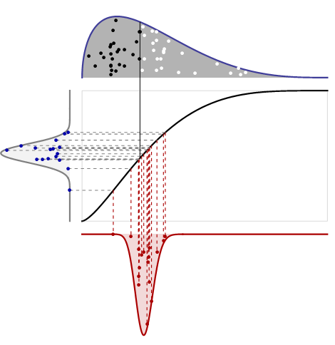
Figure 4

This looks complicated, but it's really quite simple. There are four related plots here:

  1. The top plot shows the PDF of a distribution along with one random sample of size $n$. Values greater than the median are shown as white dots; values less than the median as black dots. It does not need a vertical scale because we know the total area is unity.

  2. The middle plot is the cumulative distribution function for the same distribution: it uses height to denote probability. It shares its horizontal axis with the first plot. Its vertical axis must go from $0$ to $1$ because it represents probabilities.

  3. The left plot is meant to be read sideways: it is the PDF of the Beta$(n/2+1, n/2+1)$ distribution. It shows how the median in the box will vary, when the median is measured in terms of areas to the left and right of the middle (rather than measured by its horizontal position). I have drawn $16$ random points from this PDF, as shown, and connected them with horizontal dashed lines to the corresponding locations on the original CDF: this is how volumes (measured at the left) are converted to positions (measured across the top, center, and bottom graphics). One of these points actually corresponds to the median shown in the top plot; I have drawn a solid vertical line to show that.

  4. The bottom plot is the sampling density of the median, as measured by its horizontal position. It is obtained by converting area (in the left plot) to position. The conversion formula is given by the inverse of the original CDF: this is simply the definition of the inverse CDF! (In other words, the CDF converts position into area to the left; the inverse CDF converts back from area to position.) I have plotted vertical dashed lines showing how the random points from the left plot are converted into random points within the bottom plot. This process of reading across and then down tells us how to go from area to position.

Let $F$ be the CDF of the original distribution (middle plot) and $G$ the CDF of the Beta distribution. To find the chance that the median lies to the left of some position $x$, first use $F$ to obtain the area to the left of $x$ in the box: this is $F(x)$ itself. The Beta distribution at the left tells us the chance that half the atoms will lie within this volume, giving $G(F(x))$: this is the CDF of the median position. To find its PDF (as shown in the bottom plot), take the derivative:

$$\frac{d}{dx}G(F(x)) = G'(F(x))F'(x) = g(F(x))f(x)$$

where $f$ is the PDF (top plot) and $g$ is the Beta PDF (left plot).

This is an exact formula for the distribution of the median for any continuous distribution. (With some care in interpretation it can be applied to any distribution whatsoever, whether continuous or not.)


Asymptotic Results

When $n$ is very large and $F$ does not have a jump at its median, the sample median must vary closely around the true median $\mu$ of the distribution. Also assuming the PDF $f$ is continuous near $\mu$, $f(x)$ in the preceding formula will not change much from its value at $\mu,$ given by $f(\mu).$ Moreover, $F$ will not change much from its value there either: to first order,

$$F(x) = F\left(\mu + (x-\mu)\right) \approx F(\mu) + F^\prime(\mu)(x-\mu) = 1/2 + f(\mu)(x-\mu).$$

Thus, with an ever-improving approximation as $n$ grows large,

$$g(F(x))f(x) \approx g\left(1/2 + f(\mu)(x-\mu)\right) f(\mu).$$

That is merely a shift of the location and scale of the Beta distribution. The rescaling by $f(\mu)$ will divide its variance by $f(\mu)^2$ (which had better be nonzero!). Incidentally, the variance of Beta$(n/2+1, n/2+1)$ is very close to $n/4$.

This analysis can be viewed as an application of the Delta Method.

Finally, Beta$(n/2+1, n/2+1)$ is approximately Normal for large $n$. There are many ways to see this; perhaps the simplest is to look at the logarithm of its PDF near $1/2$:

$$\log\left(C(1/2 + x)^{n/2}(1/2-x)^{n/2}\right) = \frac{n}{2}\log\left(1-4x^2\right) + C' = C'-2nx^2 +O(x^4).$$

(The constants $C$ and $C'$ merely normalize the total area to unity.) Through third order in $x,$ then, this is the same as the log of the Normal PDF with variance $1/(4n).$ (This argument is made rigorous by using characteristic or cumulant generating functions instead of the log of the PDF.)

Putting this altogether, we conclude that

  • The distribution of the sample median has variance approximately $1/(4 n f(\mu)^2)$,

  • and it is approximately Normal for large $n$,

  • all provided the PDF $f$ is continuous and nonzero at the median $\mu.$

$\endgroup$
10
  • 8
    $\begingroup$ 'Tis a thing of beauty. $\endgroup$ Commented Mar 24, 2014 at 23:50
  • 1
    $\begingroup$ @Tim I do not understand the relevance of the reference to a prior, but I do appreciate you pointing out that the correct name of the Beta distribution identified in the "Intuition" section is Beta$(n/2+1,n/2+1)$. I'll fix that wherever it occurs (which is in several places in the discussion). $\endgroup$
    – whuber
    Commented Feb 4, 2016 at 14:57
  • 1
    $\begingroup$ I was re-reading this and thought to myself "this looks like a whuber answer". Lo and behold it was a whuber answer. $\endgroup$ Commented Sep 23, 2020 at 19:23
  • 5
    $\begingroup$ @Engr And behold--you had commented on it over six years ago! After so much time and so many posts, we easily forget so much... . $\endgroup$
    – whuber
    Commented Sep 23, 2020 at 19:33
  • 1
    $\begingroup$ @user67724 Thank you for that comment. I have had poor luck with TAS. I submitted an enhanced version of stats.stackexchange.com/a/18200/919 a couple years ago and it was rejected, without substantial review, as being too trivial. I remain open to suggestions and encouragement, though ;-). $\endgroup$
    – whuber
    Commented Sep 28, 2022 at 13:57
29
$\begingroup$

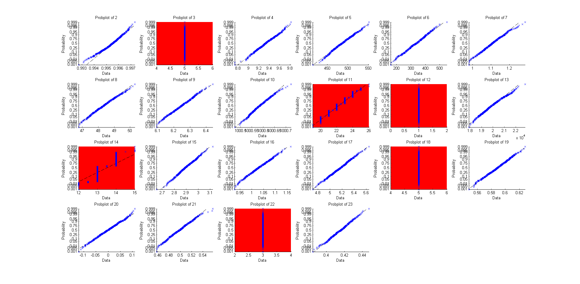
@EngrStudent illuminating answer tells us that we should expect different results when the distribution is continuous, and when it is discrete (the "red" graphs, where the asymptotic distribution of the sample median fails spectacularly to look like normal, correspond to the distributions Binomial(3), Geometric(11), Hypergeometric(12), Negative Binomial(14), Poisson(18), Discrete Uniform(22).

And indeed this is the case. When the distribution is discrete, things get complicated. I will provide the proof for the Absolutely Continuous Case, essentially doing no more than detailing the answer already given by @Glen_b, and then I will discuss a bit what happens when the distribution is discrete, providing also a recent reference for anyone interested in diving in.

ABSOLUTELY CONTINUOUS DISTRIBUTION
Consider a collection of i.i.d. absolutely continuous random variables $\{X_1,...X_n\}$ with distribution function (cdf) $F_X(x) = P(X_i\le x)$ and density function $F'_X(x)=f_X(x)$. Define $Z_i\equiv I\{X_i\le x\}$ where $I\{\}$ is the indicator function. Therefore $Z_i$ is a Bernoulli r.v., with $$E(Z_i) = E\left(I\{X_i\le x\}\right) = P(X_i\le x)=F_X(x),\;\; \text{Var}(Z_i) = F_X(x)[1-F_X(x)],\;\; \forall i$$

Let $Y_n(x)$ be the sample mean of these i.i.d. Bernoullis, defined for fixed $x$ as $$Y_n(x) = \frac 1n\sum_{i=1}^nZ_i$$ which means that $$E[Y_n(x)] = F_X(x),\;\; \text{Var}(Y_n(x)) = (1/n)F_X(x)[1-F_X(x)]$$ The Central Limit Theorem applies and we have

$$\sqrt n\Big(Y_n(x) - F_X(x)\Big) \rightarrow_d \mathbb N\left(0,F_X(x)[1-F_X(x)]\right) $$

Note that $Y_n(x) = \hat F_n(x)$ i.e. non else than the empirical distribution function. By applying the "Delta Method" we have that for a continuous and differentiable function $g(t)$ with non-zero derivative $g'(t)$ at the point of interest, we obtain

$$\sqrt n\Big(g[\hat F_n(x)] - g[F_X(x)]\Big) \rightarrow_d \mathbb N\left(0,F_X(x)[1-F_X(x)]\cdot\left(g'[F_X(x)]\right)^2\right) $$

Now, choose $g(t) \equiv F^{-1}_X(t),\;\; t\in (0,1)$ where $^{-1}$ denotes the inverse function. This is a continuous and differentiable function (since $F_X(x)$ is), and by the Inverse Function Theorem we have

$$g'(t)=\frac {d}{dt}F^{-1}_X(t) = \frac 1{f_x\left(F^{-1}_X(t)\right)}$$

Inserting these results on $g$ in the delta-method derived asymptotic result we have

$$\sqrt n\Big(F^{-1}_X(\hat F_n(x)) - F^{-1}_X(F_X(x))\Big) \rightarrow_d \mathbb N\left(0,\frac {F_X(x)[1-F_X(x)]}{\left[f_x\left(F^{-1}_X(F_X(x))\right)\right]^2} \right) $$

and simplifying,

$$\sqrt n\Big(F^{-1}_X(\hat F_n(x)) - x\Big) \rightarrow_d \mathbb N\left(0,\frac {F_X(x)[1-F_X(x)]}{\left[f_x(x)\right]^2} \right) $$

.. for any fixed $x$. Now set $x=m$, the (true) median of the population. Then we have $F_X(m) = 1/2$ and the above general result becomes, for our case of interest,

$$\sqrt n\Big(F^{-1}_X(\hat F_n(m)) - m\Big) \rightarrow_d \mathbb N\left(0,\frac {1}{\left[2f_x(m)\right]^2} \right) $$

But $F^{-1}_X(\hat F_n(m))$ converges to the sample median $\hat m$. This is because

$$F^{-1}_X(\hat F_n(m)) = \inf\{x : F_X(x) \geq \hat F_n(m)\} = \inf\{x : F_X(x) \geq \frac 1n \sum_{i=1}^n I\{X_i\leq m\}\}$$

The right-hand side of the inequality converges to $1/2$ and the smallest $x$ for which eventually $F_X \geq 1/2$, is the sample median.

So we obtain

$$\sqrt n\Big(\hat m - m\Big) \rightarrow_d \mathbb N\left(0,\frac {1}{\left[2f_x(m)\right]^2} \right) $$ which is the Central Limit Theorem for the sample median for absolutely continuous distributions.

DISCRETE DISTRIBUTIONS
When the distribution is discrete (or when the sample contains ties) it has been argued that the "classical" definition of sample quantiles, and hence of the median also, may be misleading in the first place, as the theoretical concept to be used in order to measure what one attempts to measure by quantiles.
In any case it has been simulated that under this classical definition (the one we all know), the asymptotic distribution of the sample median is non-normal and a discrete distribution.

An alternative definition of sample quantiles is by using the concept of the "mid-distribution" function, which is defined as $$F_{mid}(x) = P(X\le x) - \frac 12P(X=x)$$

The definition of sample quantiles through the concept of mid-distribution function can be seen as a generalization that can cover as special cases the continuous distributions, but also, the not-so-continuous ones too.

For the case of discrete distributions, among other results, it has been found that the sample median as defined through this concept has an asymptotically normal distribution with an ...elaborate looking variance.

Most of these are recent results. The reference is Ma, Y., Genton, M. G., & Parzen, E. (2011). Asymptotic properties of sample quantiles of discrete distributions. Annals of the Institute of Statistical Mathematics, 63(2), 227-243., where one can find a discussion and links to the older relevant literature.

$\endgroup$
7
  • 3
    $\begingroup$ (+1) For the article. This is an excellent answer. $\endgroup$ Commented Feb 18, 2014 at 15:23
  • 2
    $\begingroup$ Can you please explain why $F^{-1}_X(\hat F_n(m))$ converges to the sample median $\hat m$? $\endgroup$ Commented Oct 24, 2018 at 15:59
  • 1
    $\begingroup$ I know that $\hat F_n(m) \to F_X(m) $ in distribution, but I cannot see how sample median $\hat m$ is equal to $F^{-1}_X(\hat F_n(m))$ $\endgroup$ Commented Oct 24, 2018 at 16:13
  • 2
    $\begingroup$ @kasa I elaborated a bit on the matter. $\endgroup$ Commented Oct 25, 2018 at 23:55
  • 1
    $\begingroup$ I am sorry to keep bringing this up again: But the smallest $x$ for which eventually $F_X(x) ≥ 1/2 $, is the population median, not the sample median, isn't it? $\endgroup$ Commented Oct 26, 2018 at 8:20
14
$\begingroup$

Yes it is, and not just for the median, but for any sample quantile. Copying from this paper, written by T.S. Ferguson, a professor at UCLA (his page is here), which interestingly deals with the joint distribution of sample mean and sample quantiles, we have:

Let $X_1, . . . ,X_n$ be i.i.d. with distribution function $F(x)$, density $f(x)$, mean $\mu$ and finite variance $\sigma^2$. Let $0 < p < 1$ and let $x_p$ denote the $p$-th quantile of $F$, so that $F(x_p) = p$. Assume that the density $f(x)$ is continuous and positive at $x_p$. Let $Y_n = X_{(n:\lceil np\rceil)}$ denote the sample $p$-th quantile. Then

$$\sqrt n(Y_n − x_p) \xrightarrow{d} N(0, p(1 − p)/(f(x_p))^2)$$

For $p=1/2 \Rightarrow x_p=m$ (median), and you have the CLT for medians,

$$\sqrt n(Y_n − m) \xrightarrow{d} N\left(0, [2f(m)]^{-2}\right)$$

$\endgroup$
3
  • 2
    $\begingroup$ Nice. It is worth mentioning that the variance of the sample median is not as easy to estimate as the one for the sample mean. $\endgroup$
    – Michael M
    Commented Nov 10, 2013 at 7:30
  • 1
    $\begingroup$ @Alecos - how did you get two answers for this question? $\endgroup$ Commented Apr 19, 2017 at 15:28
  • 2
    $\begingroup$ @EngrStudent The system allows it, it just asks you to verify that you want indeed to add a second answer. $\endgroup$ Commented Apr 19, 2017 at 15:31
13
$\begingroup$

I like the analytic answer given by Glen_b. It is a good answer.

It needs a picture. I like pictures.

Here are areas of elasticity in an answer to the question:

  • There are lots of distributions in the world. Mileage is likely to vary.
  • Sufficient has different meanings. For a counter-example to a theory, sometimes a single counter-example is required for "sufficient" to be met. For demonstration of low defect rates using binomial uncertainty hundreds or thousands of samples may be required.

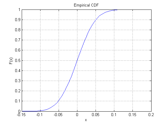
For a standard normal I used the following MatLab code:

mysamples=1000;

loops=10000;

y1=median(normrnd(0,1,mysamples,loops));

cdfplot(y1)

and I got the following plot as an output:

enter image description here

So why not do this for the other 22 or so "built-in" distributions, except using prob-plots (where straight line means very normal-like)?

enter image description here

And here is the source code for it:

mysamples=1000;

loops=600;

y=zeros(loops,23);

y(:,1)=median(random('Normal', 0,1,mysamples,loops));

y(:,2)=median(random('beta', 5,0.2,mysamples,loops));
y(:,3)=median(random('bino', 10,0.5,mysamples,loops));
y(:,4)=median(random('chi2', 10,mysamples,loops));
y(:,5)=median(random('exp', 700,mysamples,loops));

y(:,6)=median(random('ev', 700,mysamples,loops));
y(:,7)=median(random('f', 5,3,mysamples,loops));
y(:,8)=median(random('gam', 10,5,mysamples,loops));
y(:,9)=median(random('gev', 0.24, 1.17, 5.8,mysamples,loops));
y(:,10)=median(random('gp', 0.12, 0.81,mysamples,loops));

y(:,11)=median(random('geo', 0.03,mysamples,loops));
y(:,12)=median(random('hyge', 1000,50,20,mysamples,loops));
y(:,13)=median(random('logn', log(20000),1.0,mysamples,loops));
y(:,14)=median(random('nbin', 2,0.11,mysamples,loops));
y(:,15)=median(random('ncf', 5,20,10,mysamples,loops));

y(:,16)=median(random('nct', 10,1,mysamples,loops));
y(:,17)=median(random('ncx2', 4,2,mysamples,loops));
y(:,18)=median(random('poiss', 5,mysamples,loops));
y(:,19)=median(random('rayl', 0.5,mysamples,loops));
y(:,20)=median(random('t', 5,mysamples,loops));

y(:,21)=median(random('unif',0,1,mysamples,loops));
y(:,22)=median(random('unid', 5,mysamples,loops));
y(:,23)=median(random('wbl', 0.5,2,mysamples,loops));


figure(1); clf
hold on

for i=2:23
    subplot(4,6,i-1)

    probplot(y(:,i))
    title(['Probplot of ' num2str(i)])
    axis tight

    if not(isempty(find(i==[3,11,12,14,18,22])))
        set(gca,'Color','r')
    end

end

When I see the analytic proof I might think "in theory they all might fit" but when I try it out then I can temper that with "there are a number of ways this doesn't work so well, often involving discrete or highly constrained values" and this might make me want to be more careful about applying the theory to anything that costs money.

Good luck.

$\endgroup$
2
  • 1
    $\begingroup$ Am I wrong or the distribution for which the median is not normally distributed are discrete? $\endgroup$
    – SeF
    Commented Mar 19, 2019 at 19:00
  • 2
    $\begingroup$ @SeF - some of the other answers are very illuminating here. $\endgroup$ Commented Sep 15, 2020 at 14:24

Your Answer

By clicking “Post Your Answer”, you agree to our terms of service and acknowledge you have read our privacy policy.

Not the answer you're looking for? Browse other questions tagged or ask your own question.