What to do if the rate of misclassification in Bayesian model selection depends on the model parameter

Question

I am currently having problems with a Bayesian model selection where the rate of misclassification seems to depend on the actual model parameter. I can create a simple minimal example of this effect, and I can understand why this happens, but I am not sure how to rectify this problem. Here is a minimal example:

1. Assume two measurements $K_1 \sim Binom(v_1,N)$ and $K_2 \sim Binom(v_2,N)$.
2. The question I am interested in is whether $v_1 = 1-v_2$ or if these two variables are independent.
3. Thus I have two models, one as above (with two parameters $\theta_{1,2}$ and the other is given by $(K_1+K_2) \sim Binom(\theta,2N)$.

Assuming flat priors on the parameters and equal prior likelihood for both models, I can derive the Bayes factor as

$BF_{1,2}=\frac{B(N+K_1-K_2+1,\;N+K_2-K_1+1)}{B(K_1+1,\;N-K_1+1)B(K_2+1,\;N-K_2+1)}.$

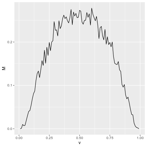
However, when I simulate this only with the model where $v_1=1-v_2$, I find that the rate of misclassification depends strongly on the actual probability I use in the simulation:

library(tidyverse)
library(ggplot2)

N <- 10

reps <- 1000

BF12 <- function(k1,k2,N) {
  beta(N-k2+k1+1,N-k1+k2+1)/(beta(k1+1,N-k1+1)*beta(k2+1,N-k2+1))
}

v <- seq(0.01,0.99,by=0.01)

df <- expand.grid(v = v, i = seq_len(reps))

df$K1 <- map_dbl(df$v,function(v) rbinom(1,N,v))
df$K2 <- map_dbl(df$v,function(v) rbinom(1,N,1-v))

df$BF <- BF12(df$K1,df$K2,N)

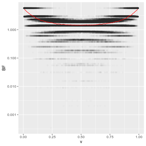
ggplot(df,aes(x=v,y=BF)) + 
  geom_jitter(alpha=0.01) + 
  geom_line(data=df %>% group_by(v) %>% summarize(BF=mean(BF)), color="red") + 
  scale_y_log10()


df %>% group_by(v) %>% summarize(M=mean(BF < 1)) %>% ggplot(aes(x=v,y=M)) + geom_line()

Bayes factors:

Rate of Misclassification:

It is clear, why this happens. If the parameter becomes closer to $0.5$, then these two models become indeed more similar to each other. However, is there any method to rectify this problem?

Additional details:

This problem appears as part of a broader analysis. In the complete analysis, I actually have two models, similar to $v_1=1-v_2$ vs. $v_1=v_2$ and I want to distinguish between those two models using MCMC. Because I am not sure these two models adequately describe my data, I also added a model where $v_1$ and $v_2$ are independent (basically to leave those examples as unclassified). However, during analysis, I found that the parameters are distributed differently for the two groups, so I have a higher rate of misclassification (as unclassified) in one of the groups vs. the other group.

EDIT

Some more details on why I think this happens:

While in general one could just take this to be some kind of "identifiability issue", I don't think this adequately describes my problem. Of course, the more general two-parameter model can easily mimic the simpler model (they are nested), but in that case, the simpler model should be preferred because BF controls for model complexity. However, that only would explain, why the simpler model is chosen for some data produced by the more complex model (which is actually what I want, so not a problem), but not vice versa as in my example.

Rather, it seems that for some parameters of the simpler model, the data itself becomes less indicative of any of the models. This also seems to be specifically related to the use of binomially distributed variables here, because in the case of the simpler model the variance increases when $v$ approaches $0.5$.

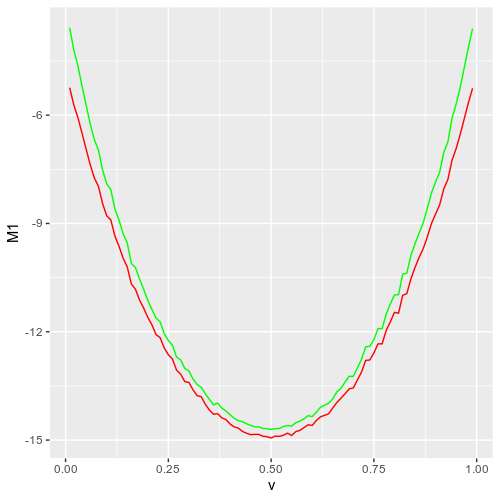
If I plot the posterior log-odds for each model, it becomes more clear what is happening here:

Both models become less likely as $v$ approaches $0.5$, but the drop is stronger for the simpler model, leading to a decrease of the BF.

Answer 1

However, is there any method to rectify this problem?

No, for the simple reason that this is not a problem, but a property of your models. Let's have a look at Figure 2-A (left panel) of the following paper. We have 2 models:

• A model called "binomial", which is a mixture of several Gaussians;
• A model called "gaussian", which is just one Gaussian distribution.

The binomial model has several parameters, including a value $\sigma$ (which is the variance of each Gaussian in the mixture, and hence the width of each "peak" you see in the figure). If $\sigma$ becomes too high, the peaks in the binomial model will overlap, and it will become very similar to a Gaussian distribution, and data generated from the binomial will be misclassified (the Gaussian model will provide a better fit).

That's very similar to your situation, where for $v$ close to 0.5, the complex model (with more parameters) becomes indistinguishable from the simpler model. However, the identifiability of a model is a function not only of its parameters, but also of the experimental protocol (i.e. the number of data points). Intuitively, if you increase the number of data points in your samples, the missclassification shall decrease (although it will remain peaky around 0.5)

You might find the following papers interesting:

Acerbi, L., Ma, W. J., & Vijayakumar, S. (2014). A framework for testing identifiability of Bayesian models of perception. In Advances in neural information processing systems (pp. 1026-1034).

Navarro, D. J., Pitt, M. A., & Myung, I. J. (2004). Assessing the distinguishability of models and the informativeness of data. Cognitive psychology, 49(1), 47-84.

Daw, N. D. (2011). Trial-by-trial data analysis using computational models. Decision making, affect, and learning: Attention and performance XXIII, 23(1).

I myself am working on this subject for my PhD project. Happy to discuss it any further !

EDIT

I took the problem in the wrong way in my answer: I looked at how data generated from a complex model are correctly classified compared to a simple model. Here, the question is why are some data generated from a simple model misclassified as being generated from a complex model.

The intuition is indeed that, on average, data generated from a simple model should not be misclassified and attributed to a more complicated model. Indeed, both models, the simple and the complex, are going to fit data equally well, but the Bayes Factor is going to favor the simpler one. I insist on the on average: it is still possible that a simple model will, from time to time, generate weirdly distributed data for which a complex model will provide a very good fit. But that is unlikely, so on average, if data are generated from a simple model, then model selection will choose the simple model.

I tried to obtain a formal proof for this intuition : Formal proof of Occam's razor for nested models

I think that is indeed what you observe on your first plot: while some data are misclassified, on average the BF is > 1.