Does $cov(x,y)=cov(x,x)=cov(y,y)$ imply $x=y$?

Question

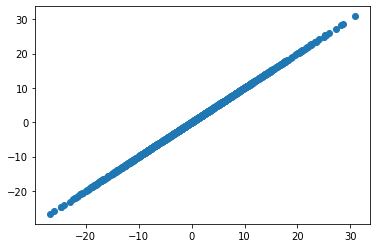
Given two random variables, you can calculate their covariance matrix. I noticed that if I plot data (in my case multi-variate normal) coming from a cov-matrix whose elements are all the same, e.g.

$\begin{pmatrix} 100 & 100 \\ 100 & 100 \end{pmatrix}$

You will get a straight line. e.g. in python:

data = np.random.multivariate_normal([0,0], [[100,100],[100,100]], 1000)
plt.scatter(data[:,0], data[:,1])

I wonder if this implies that $x=y$?

Also, can there be a case where $cov(x,y) = cov(x,x) \ne cov(y,y)$ and if so, is there any insight about what's going on there?

Answer 1

Not quite. As an example, take

$$ X\sim\mathcal{N}(0, 100) \\ Y = X+3, $$

or, equivalently,

$$ \left[\begin{array}{c} X \\ Y\end{array}\right]\sim\mathcal{N}\bigg(\left[\begin{array}{c} 0 \\ 3\end{array}\right], \left[\begin{array}{cc} 100 & 100 \\ 100 & 100\end{array}\right]\bigg). $$

Then we have $Var(X) = Var(Y) = Cov(X, Y) = 100$, but $X$ and $Y$ are not equal ($Y$ is always 3 larger than $X$).

Though this example shows that $Var(X)=Var(Y)=Cov(X,Y)$ does not imply $X=Y$, it does imply (with probability 1) that $X$ and $Y$ differ by some constant $c$. The covariance matrix can't be used to determine what that constant is -- you would need to know the means as well to learn the constant.

---

To your second question, it is quite common to have $Var(X) = Cov(X, Y) \neq Var(Y)$, and there's nothing particularly special about this situation. All that it represents is two random variables with different variances and a moderate amount of correlation. For instance, the following are two normal random variables with different variances and a correlation of 0.1.

$$ \left[\begin{array}{c} X \\ Y\end{array}\right]\sim\mathcal{N}\bigg(\left[\begin{array}{c} 0 \\ 0\end{array}\right], \left[\begin{array}{cc} 1 & 1 \\ 1 & 100\end{array}\right]\bigg). $$

Answer 2

Hint: $$Var(X-Y)=Var(X)+Var(Y)-2cou(X,Y)$$

and $Var(X-Y)=E\bigg((X-Y)-E(X-Y)\bigg)^2=0$

so $P\{(X-Y)-E(X-Y)=0\}=1$ so $X-Y$ almost surly constant

Answer 3

I want to discuss why you observed all the data on the particular line that you did.

---

$\newcommand{\1}{\mathbf 1}$If you have a random variable $X \sim \mathcal N(\mathbf 0, \Sigma)$ where $\Sigma$ has all the same element, then $\Sigma \propto \1\1^T$ so you have a rank $1$ covariance matrix.

I'll consider the more general problem of what it means to have a multivariate Gaussian with a low-rank covariance matrix. Suppose $X \sim\mathcal N_p(\mathbf 0, \Sigma)$ and $1 \leq \text{rank}(\Sigma) := r < p$. We can factor $\Sigma$ as $$ \Sigma = \tilde Q\tilde \Lambda \tilde Q^T $$ via the spectral theorem with $\Lambda = \text{diag}(\lambda_1,\dots,\lambda_r, 0, \dots, 0)$. This means that $\Sigma$ can actually be represented as $$ \Sigma = Q\Lambda Q^T $$ where $Q$ is the first $r$ columns of $\tilde Q$ and $\Lambda = \text{diag}(\lambda_1,\dots,\lambda_r)$ contains the non-zero eigenvalues.

Let $Z \sim \mathcal N_r(\mathbf 0, I)$ and define $$ Y = Q\Lambda^{1/2}Z. $$ $Y$ is a linear transformation of a Gaussian so it too is Gaussian, and $$ \text{E}(Y) = \mathbf 0 \\ \text{Var}(Y) = Q\Lambda^{1/2}\Lambda^{1/2}Q^T = \Sigma $$ so $Y \sim \mathcal N(\mathbf 0, \Sigma) \stackrel{\text d}= X$.

This shows that we can think of $X$ as being generated by a low dimensional Gaussian that we map up into our high dimensional space, and this explains why there is still randomness but not over all of $\mathbb R^p$. In particular, $X$ is constrained to the $r$-dimensional column space of $Q$.

In your case we have $\Sigma \propto \1\1^T$ which means that $r=1$ and $Q = p^{-1/2}\mathbf 1$. This shows that $X \in \text{span}(\1)$ which is what you observed.

---

One final comment: these Gaussians with low-rank covariance matrices do not have pdfs in the usual sense because $P(X \in \text{ColSpace}(Q)) = 1$ yet the Lebesgue measure of $\text{ColSpace}(Q)$ is zero w.r.t. the Lebesgue measure on $\mathbb R^p$. This is one advantage to defining a multivariate Gaussian as a random variable where every linear combination is Gaussian since then there's no issue with zero determinant covariance matrices in the expression for the usual pdf.