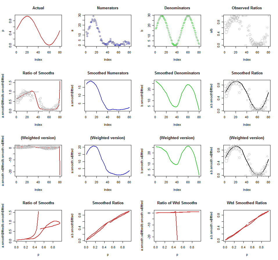
It would be erroneous to compute the ratios of the smoothed counts, because it's possible many of the ratios would not be true proportions--they could (easily) wind up outside the valid range from $0$ to $1$. (This happens in the example described below.)
Since the denominators $b_t$ vary substantially, and a count based on such a denominator typically has a variance proportional to the denominator, you should consider making weighted smooths of the ratios using the $b_t$ as the weights.
To study this, I created time series $a_t$ and $b_t$ which vary substantially and are temporally correlated. The $a_t$ have binomial distributions based on the counts in $b_t$, with regularly (sinusoidally) varying probabilities. These, and their ratio $a_t/b_t$, are shown in the first row of the figure below. (The dots for the observations are scaled so their areas are proportional to $b_t$: larger dots represent more reliable data.) Then I compute four possible smooths: the ratio of the smooths, the smoothed ratio, and the two weighted versions. These occupy the next two rows: one for the unweighted version and another for the weighted version. Finally, the bottom row shows scatterplots of these four smooths against the true probabilities.
In experimenting with various values of n (length of series, ranging from $40$ to $200$) and m (maximum possible value of $b_t$, ranging from $3$ to $600$), I find the weighted smoothed ratio is slightly--but visibly--better than the unweighted smoothed ratio, and both are consistently much better than the ratios of the smooths (weighted or not). Compare the bottom right scatterplot ("Wtd Smoothed Ratios") to its unweighted counterpart, second from the left at the bottom ("Smoothed Ratios"). Ideally, these plots would be diagonal lines. Notice the wild behavior of the ratios of smooths and their extreme departures from the ideal. That awfulness is equally apparent in the plots of smooths against the data shown in the first column (second and third rows).

n <- 80
m <- 30
z <- 1.1
p <- (1 + sin(2 * pi * 1:n / n)) / (1+z)
q <- (1 + sin(5/3 * 2 * pi * 1:n / n)) / (1+z)
b <- ceiling(0.001 + m * q)
scale <- sqrt(b/m)*3
set.seed(26)
a <- rbinom(n, b, p)

col = c(rgb(.8,.2,.2), rgb(.2,.2,.8), rgb(.2,.8,.2), "Black", "Gray")
par(mfrow=c(4,4))
plot(p, type="l", lwd=2, col=col[1], main="Actual")
plot(a, col=col[2], main="Numerators")
plot(b, col=col[3], main="Denominators")
plot(a/b, col=col[5], main="Observed Ratios", cex=scale)

a.smooth <- loess(a ~ as.vector(1:n))
b.smooth <- loess(b ~ as.vector(1:n))
a.b.smooth <- loess(a/b ~ as.vector(1:n))

plot(a.smooth$fitted / b.smooth$fitted, col=col[1], type="l", lwd=2,
     main="Ratio of Smooths")
points(a/b, col=col[5], cex=scale)
plot(a.smooth$fitted, col=col[2], type="l", lwd=2, main="Smoothed Numerators")
plot(b.smooth$fitted, col=col[3], type="l", lwd=2, main="Smoothed Denominators")
plot(a.b.smooth$fitted, col=col[4], type="l", lwd=2, main="Smoothed Ratios")
points(a/b, col=col[5], cex=scale)

a.smooth.w <- loess(a ~ as.vector(1:n), weights=b)
b.smooth.w <- loess(b ~ as.vector(1:n), weights=b)
a.b.smooth.w <- loess(a/b ~ as.vector(1:n), weights=b)

plot(a.smooth.w$fitted / b.smooth.w$fitted, col=col[1], type="l", lwd=2,
     main="(Weighted version)")
points(a/b, col=col[5], cex=scale)
plot(a.smooth.w$fitted, col=col[2], type="l", lwd=2, main="(Weighted version)")
plot(b.smooth.w$fitted, col=col[3], type="l", lwd=2, main="(Weighted version)")
plot(a.b.smooth.w$fitted, col=col[4], type="l", lwd=2, main="(Weighted version)")
points(a/b, col=col[5], cex=scale)

plot(p, a.smooth$fitted / b.smooth$fitted, col=col[1], type="l", lwd=2,
     main="Ratio of Smooths")
plot(p, a.b.smooth$fitted, col=col[1], type="l", lwd=2, main="Smoothed Ratios")
plot(p, a.smooth.w$fitted / b.smooth.w$fitted, col=col[1], type="l", lwd=2,
     main="Ratio of Wtd Smooths")
plot(p, a.b.smooth.w$fitted, col=col[1], type="l", lwd=2,
     main="Wtd Smoothed Ratios")

