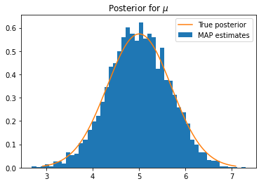
I've recently read interesting paper Uncertainty in Neural Networks: Approximately Bayesian Ensembling by Pearce et al (2020), who suggested algorithm for approximating the posterior distribution by taking sample from the prior $\theta_{acc} \sim p(\theta)$ and finding MAP estimate using
$$ \theta_\text{MAP}' = \underset{\theta}{\operatorname{arg\,max}} \; p(x | \theta) \; p_{acc}(\theta) $$
where $p_{acc}(\theta)$ is the prior distribution centred at the $\theta_{acc}$ value. This is repeated many times, and we treat the ensemble of such estimates as samples from the posterior distribution.
Unfortunately, the above approach underestimates the variability of the parameters. What if instead we varied the data, rather then priors? We could take bootstrap sample $x^*$ from the data $x$ and then estimate
$$ \theta_\text{MAP}^* = \underset{\theta}{\operatorname{arg\,max}} \; p(x^* | \theta) \; p(\theta) $$
again, repeating this many times, and ensembling the results. My questions:
- Do you recall anyone describing such approach? So far, the closest I found is the paper by Laird and Louis (1985) about combining empirical Bayes with bootstrap.
- What could be the potential problems with this approach? Why could it, or could not work?
Doing this for a trivial example of estimating mean of normal distribution with known variance gives pretty nice results.
import numpy as np
import matplotlib.pyplot as plt
import scipy.stats as sp

np.random.seed(42)

n = 15
# true parameters
μ = 5
σ = 2.7

x = sp.norm(μ, σ).rvs(n)

prior_μ = 0
prior_σ = 10
prior_dist = sp.norm(prior_μ, prior_σ)

def posterior(x, prior_μ, prior_σ):
    n = len(x)
    σ2 = σ ** 2
    prior_σ2 = prior_σ ** 2

    post_σ2 = 1 / (1/prior_σ2 + n/σ2)
    post_μ = post_σ2 * (prior_μ/prior_σ2 + np.sum(x)/σ2)

    return float(post_μ), np.sqrt(post_σ2)

post_μ, post_σ = posterior(x, prior_μ, prior_σ)
post_dist = sp.norm(post_μ, post_σ)

R = 5000
results = []

for _ in range(R):
    idx = np.random.choice(n, n, replace=True)
    results.append(posterior(x[idx], prior_μ, prior_σ))

results = np.vstack(results)

np.mean(results[:, 0]), np.std(results[:, 0])
## (4.9949681628669085, 0.6582492996849297)

# vs true posterior
post_μ, post_σ
## (5.003623405947105, 0.6954491092861294)


