Goodness of Fit ot Least Squares with known measurement uncertainty

Question

We want to estimate $\beta$ for $$ y = x\beta + \epsilon $$ where $y$ and $x$ are $n\times 1$ vector and $\epsilon$ is not i.i.d, but $\epsilon \sim N(0, \sigma^2\Omega)$, where $\Omega$ and $W$ are $n \times n$ nonsingular, positive definite and symmetric matrix with $W_{ii}=w_i=\frac{\sigma^2}{\sigma_i^2}$ and $\Omega_{ii}=\frac{1}{\sigma_i^2}$ .

Assume that, thanks to a lot of repeated measurements, we know the underlying measurement uncertainties $\sigma_i$ of my response variable in the i-th measured point, so $\Omega$ and $W$ are known. We measure a total of $n$ points.

Given Heteroskedasticity we use weigthed least squares.

The residual analysis yields good results, showing that the residuals are independent and normally distributed, and that the weights enable studentized residuals with constant variance.

Now what is the best way to assess the goodness of fit ?

1.) Reduced chi-square: $\chi_{red}^2$ should be close to 1. (1) (2) $$\chi_{red}^2 = \frac{\chi^2}{\nu} = \frac{r'\Omega r}{\nu} = \frac{1}{\nu} \cdot \sum_i^n\frac{ r_i^2}{\sigma_i^2} $$

N.B.: This corresponds to a comparison of the unbiased estimate of error variance $\hat{\sigma}^2$ and the known mean measurement uncertainty $\sigma^2$. $$ \frac{\hat{\sigma}^2}{\sigma^2} = \frac{r'\Omega r}{\nu} \cdot \frac{1}{\sigma^2} = \frac{ \frac{1}{\nu} \sum_i^n r_i^2 \cdot w_i}{\sigma^2} = \frac{ \frac{1}{\nu} \sum_i^n r_i^2 \cdot \frac{\sigma^2}{\sigma_i^2}}{\sigma^2} = \frac{1}{\nu} \cdot \sum_i^n\frac{ r_i^2}{\sigma_i^2} $$

or

2.) Evaluation of the variance of the standardized/studentized Residuals, which should be close to 1. Note that the value for $\sigma$ would be the one geven by the prior repeated measurements and not the MSE, where:

Standardized Residuals $\sim \mathcal{N}(0,\,1)$, so $Var(r_{i,Stand}) \approx 1$ $$r_{i,Stand} = \frac{r_i}{\sigma_i}$$ Internally studentized Residuals: $$ r_{i,ExtStud} = \frac {r_i}{var(r_i)} = \frac{r_i}{\sqrt{\sigma^2 (\frac{1}{w_{i}} - H_{ii})}}$$

Edit: I removed the externally studentized Residuals given that I use a value of $\sigma$ that is not based on the residuals.

or another alternative ?

Answer 1

Goodness of fit is usually meant as an expression to test whether the model is sufficiently likely to be not too incorrect.

If the description of your data and the parametrization is correct, then $\chi^2$ minimization allows of the strongest tests that exists. It consists of two parts:

1. analyze the distribution of the standardized residuals as you mentioned; if these follow a standard normal distribution you have a (close to) perfect description of your parameters and their variation
2. (if possible) check whether the integrated (reduced) $\chi^2$ distribution value of repeated measurements has uniform distribution

Each of these tests on its own is extremely powerful, and in combination they are basically ensuring that your model is 'right' (unfortunately I can't find the written proof; will post this as soon as I have it again).

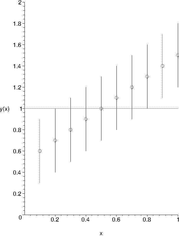
The "standard" $\chi^2$ goodness of fit test is rather weak. If the normalized $\chi^2$ is about 1, then you might not be wrong. If it is far away from 1, you also might be wrong and it might give you an indication, what is wrong. There are these hand-waving guidelines. If the value is very large, the variances might be underestimated. If the value is too small, then you may have overestimated the variances. As a counterexample consider the following graph:

I chose a constant model, and the $\chi^2$ value over the number of degrees of freedom is exactly 1. But clearly this will yield no hint to the fact that the model is wrong. If you look at the distribution of residuals, it's immediately clear that it's wrong.

Regarding the properties of the estimator (as mentioned in the comment), this can become a lot more work. The bias $b$ is the difference between the expectation value of your estimator $\hat{\beta}$ and the true value $\beta_0$. $$b=E[\hat{\beta}] - \beta_0$$ If you don't know the true value, then you'd have to find an approximation, e.g. by numerical simulation. In the sense that you have a simulated true value, reversely apply the model including the uncertainties and extract your estimation from this. Do this many times and check whether the difference is consistent with zero. The efficiency of your estimator is the ratio of the minimally possible variance of any estimator to the variance of your estimator. For single parameters the minimum variance has an expression by the Rao-Cramer-Frechet bound. Examples for this can be found in graduate course text books. For multiple parameters this becomes a lot more complicated. A first glance without the practical implications can be taken at the wikipedia entry