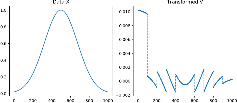
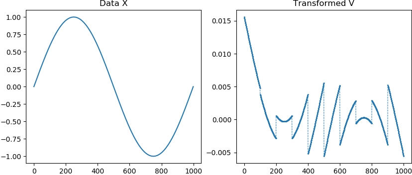
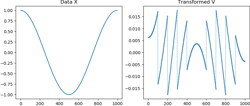
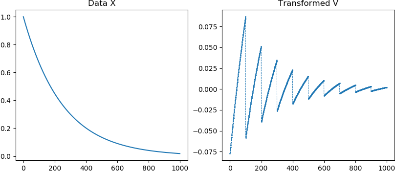
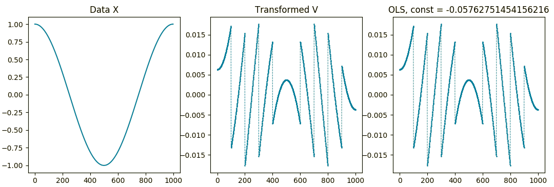
I came across this specific data transformation in the context of a physics application, which by itself is rather complex and hence out of the scope of this question. However since this transformation is applicable to general data sets, I wondered if there's a way to describe general properties of or to interpret this specific data transformation.
Suppose a set of $N$ data points $\{x_1, \ldots, x_N\}$ where $N = m\cdot n$ for two integer numbers $m, n > 1$. Then the transformation from $x_i$ to $v_i$ is given by the following system of linear equations (with $m+1$ rows and $m\cdot n$ columns):
$$ \begin{pmatrix} 1 & \cdots & 1 & 0 & \cdots & 0 & \cdots\cdots & 0 & \cdots & 0 \\ 0 & \cdots & 0 & 1 & \cdots & 1 & \cdots\cdots & 0 & \cdots & 1 \\ \vdots & & \vdots & \vdots & & \vdots & & \vdots & & \vdots \\ 0 & \cdots & 0 & 0 & \cdots & 0 & \cdots\cdots & 1 & \cdots & 1 \\ x_{1} & \cdots & x_{n} & x_{n+1} & \cdots & x_{2n} & \cdots\cdots & x_{(m-1)\cdot n+1} & \cdots & x_{m\cdot n} \end{pmatrix} \cdot \begin{pmatrix} v_1 \\ \vdots \\ \vdots \\ \vdots \\ v_{m\cdot n} \end{pmatrix} = \begin{pmatrix} 1 \\ 0 \\ \vdots \\ 0 \\ 0 \end{pmatrix} $$
The first $m$ rows of the above coefficient matrix $A$ can be described as follows:
$$ A_{i,j} = \begin{cases} 1 \quad \textrm{if} \;\; (i-1)\cdot n < j \leq i\cdot n \\ 0 \quad \textrm{otherwise} \end{cases} $$
for $i, j \in \{1, \ldots N\}$. The last row of $A$ simply holds all the data points $x_i$. The r.h.s. vector $b$ is all zeros except for the first row which equals $1$ (in fact any other row except the last one could be chosen to hold the $1$; it's important that there is only one non-zero entry though).
This represents an underdetermined system of linear equations for which a solution can be found by minimizing the L2-norm. The solution $V^{\ast}$ is then given by the following $N\times N$ system of equations:
$$ A^T A V^{\ast} = A^T b $$
where $A^T$ is the transpose of $A$ and $b$ is the r.h.s. vector of the original system of equations. The solution $V^{\ast}$ can be found as the least-squares solution by pseudo-inversion of the matrix $A^T A$ via singular value decomposition.
Now what I'm interested in are general properties of this transformation and how the transformed data $v_i$ reflects the original data $x_i$. Even when describing all of the involved steps, I'm having difficulties interpreting the results.
Example application
This is some sample Python code which applies the above transformation to different data sets (Gaussian, sin, cos, exp).
import matplotlib.pyplot as plt
import numpy as np

m = 10
n = 100
N = m*n

x = np.exp(-np.linspace(-2, 2, N)**2)
# x = np.sin(np.linspace(0, 2*np.pi, N))
# x = np.cos(np.linspace(0, 2*np.pi, N))
# x = np.exp(-np.linspace(0, 4, N))

A = np.zeros((m+1, N))
for i in range(m):
    A[i, i*n:(i+1)*n] = 1
A[-1, :] = x

b = np.zeros(m+1)
b[0] = 1

v, *info = np.linalg.lstsq(A, b, rcond=None)

fig, (ax1, ax2) = plt.subplots(ncols=2, figsize=(10, 4))
ax1.set_title('Data X')
ax1.plot(x)
ax2.set_title('Transformed V')
ax2.plot(v, '--o', lw=0.7, ms=1)

plt.show()

