How do you fix one slope coefficient in an interaction term?

Question

hoping someone can help me with what (on the face of it) appears to be a relatively simple problem but which I can't current code out.

Basically, I would like to fit a GLM in R with a simple two-way interaction between a two-level factor and a continuous covariate, but fix the slope coefficient for one of the factor levels to be zero (while still estimating its intercept). I want to apply the method to a piecewise regression on count data (y) where for a priori reasons we 'know' there is no relationship between y and x at values of x > k but that there is a relationship at x < k. The aim is to find k by iteratively searching for the value that gives the lowest mean square error in the fitted GLMs. A simple reprex below.

First simulate some data.

set.seed(5)
k = 7
x = runif(30,0,20)                   # Simulate some values of x
y = ifelse(x<k,-0.2*x+3.5,0*x+1)     # Calculate y on scale of linear predictor
y = exp(y)                           # Convert to response scale
y = sapply(y,function(i) rpois(1,i)) # Generate some counts
plot(y~x)

Now fit a GLM using a factor to identify whether x is greater or less than k

data = data.frame(y=y,x=x,fac= x<k)
model = glm(y ~ fac + x:fac,family='poisson',data=data)
summary(model)

Coefficients:
            Estimate Std. Error z value Pr(>|z|)    
(Intercept)  1.17370    0.55206   2.126   0.0335 *  
facTRUE      2.59354    0.59167   4.383 1.17e-05 ***
facFALSE:x  -0.01833    0.03822  -0.479   0.6316    
facTRUE:x   -0.25126    0.05456  -4.605 4.12e-06 ***
---
Signif. codes:  0 ‘***’ 0.001 ‘**’ 0.01 ‘*’ 0.05 ‘.’ 0.1 ‘ ’ 1

The model does a pretty good job at recreating the coefficients used to simulate the data. However, it would probably improve the performance of the subsequent search to find k if I could fix the slope coefficient for facFALSE:x to be zero. Normally I would use an offset term for this but I can't work out how to apply it to just one level of the factor. I know there are other solutions to doing this type of segmented regression using various R packages but for my application it would be beneficial to be able to code it from first principles in this way. I'm sure there is a simple solution so any pointers gratefully received.

Thanks!

Answer 1

If you want a probabilistic inference on the location of $k$ (the change point), mcp is well suited for cases like this. It infers the parameters of change point models using Bayesian Inference (see details here).

First, let's set things up:

df = data.frame(x, y)
library(mcp)

Now we specify the two-segment model you have in mind (two formulas):

model = list(
  y ~ 1 + x,  # Intercept and slope
  ~ 0  # Joined flat line
)

Then we fit it as a poisson model and plot it:

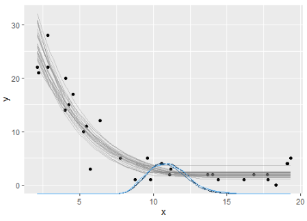
fit = mcp(model, data = df, family = poisson())
plot(fit)

The blue curves are the posterior distributions of the change point.

mcp contains many functions to summarise and check (summary(fit), pp_check(fit)), predict (fitted(fit), predict(fit)), hypothesis test (hypothesis(fit, "cp_1 > 10")), etc. on this fit. See the mcp website for more: https://lindeloev.github.io/mcp/

---

INITIAL ANSWER: If the intercept should be allowed to change at the change point, this could be your model:

model = list(
  y ~ 1 + x,  # Intercept and slope
  ~ 1  # Intercept only (flat line)
)

We use the prior to set the constraint that the second intercept can only be a negative change relative to segment 1. It's a Normal(0, 1) which is truncated to maximally be the value of segment 1 (int_1 is the intercept; x_1 is the slope on x) at the change point (cp_1):

prior = list(int_2 = "dnorm(0, 1) T(, int_1 + x_1 * cp_1)")
fit = mcp(model, data = df, prior = prior, family = poisson(), iter = 5000)
plot(fit)

Notice the weird shape which is definitely non-normal. This is much richer than least-squares methods. Change points often have these kinds of distributions because they largely depend on just a few data points in their vicinity.

Answer 2

As you write, what you really have is a "piecewise Poisson regression". Yes, it can be expressed as an interaction, but that is IMO not the best way of thinking about it, kind of calling a bike a "wheeled vehicle".

Unfortunately, the segmented package for R does not deal with Poisson regression (though it may be useful for a quick approximation using a segmented OLS model), so we will roll our own.

The simplest way would be to not use your predictor x, but to regress your Poisson response on a transformed predictor, like this:

xk <- pmin(x-k,0)
mod <- glm(y~xk,family='poisson')

Note how if x>k, we have xk==0, so your model turns into an intercept-only model, but if x<k, the model is equivalent to y~x, intercept and slope.

We can plot the response (note how the downward slope is bent, because we are plotting on the response scale, not the link scale):

x_pred <- seq(min(x),max(x),.01)
xk_pred <- pmin(x_pred-k,0)

plot(y~x)
lines(x_pred,predict(mod,newdata=data.frame(xk=xk_pred),type="response"),col="red")

Incidentally, I would not choose the value of k using in-sample squared residuals. That can lead to overfitting. Better do this by cross-validation, e.g., leave-one-out cross validation - your sample should be small enough to handle this, if your example is of the same size.