Regression in Causal Inference

Question

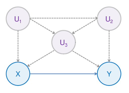
I was recently introduced to the topic of causal inference in statistics and I am currently learning about the importance of the backdoor criterion (BDC), as applied to the following DAG. Interest lies in assessing the causal effect of the treatment $X$ upon the outcome $Y$. It is easily established that the sets of variables $\lbrace U_1, U_3\rbrace$, $\lbrace U_2, U_3\rbrace$ and $\lbrace U_1, U_2, U_3\rbrace$ both satisfy the requirements of the BDC.

My confusion lies in understanding how a causal effect is modeled. Often I have seen references to OLS regression and regression with inverse probability weighting (IPW). However, I have seen very little in the way of literature describing how these can be applied to a situation such as that described in the DAG below, what conditioning on variables (or sets of variables) means in a regression model and indeed how to establish which of the three sets of variables given above should be conditioned on.

A concise explanation of the above concepts as applied to an example DAG, such as the one I have given would be very much appreciated.

Answer 1

Just to add to the excellent answers by Adrian and Noah, there is the residual question of:

how to establish which of the three sets of variables given above should be conditioned on.

Fist let's recap how the backdoor criterion is applied to this particular DAG, which I'm reposting here:

Usually we are interested in the "average causal effect" (ACE) which is the expected increase of $Y$ for a unit change in $X$. This means that we must allow all causal paths between $X \rightarrow Y$ to remain open but we must block any backdoor paths from $Y \rightarrow X$

What makes this DAG quite intriguing is that $U_3$ appears to be a confounder for $X \rightarrow Y$ but is also a collider (having 2 direct causes, $U_1$ and $U_2$). So a simplistic approach would be to say that we need to condition on it to block the backdoor path $Y \leftarrow U_3 \rightarrow X$) but then we don't want to condition on it, because that will open up the backdoor path $Y \leftarrow U_2 \rightarrow U_3 \leftarrow U_1 \rightarrow X$. This is easily resolved by blocking that path by additionally conditioining on either $U_2$ or $U_1$, or indeed both.

Thus we have arrived at the 3 candidate adjustment sets $\lbrace U_1, U_3\rbrace$, $\lbrace U_2, U_3\rbrace$ and $\lbrace U_1, U_2, U_3\rbrace$.

All 3 sets will give us an unbiased estimate of the causal effect, so how do we choose between them ?

We could reject the larger set $\lbrace U_1, U_2, U_3\rbrace$ on two grounds. First model parsimony. Second $U_2$ and $U_3$ are correlated and this correlation could be very high leading to instabilty in the estimation procedure that is used to fit the model. If they are not highly corrrelated then we might still consider this set, but with the additional considerations as below:

• we choose the set which gives us the most precise estimate of the causal effect - in a multivariable regression model this would be the estimate with the smallest standard error.

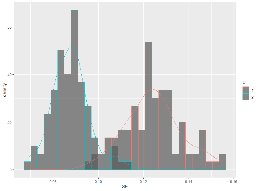
• $\lbrace U_2, U_3\rbrace$ will yield the most precise estimate because conditional on them, $U_1$ is an instrument and therefore should not be adjusted for. Adjusting for $U_2$ would reduce the residual variance of $Y$ more than adjusting for $U_1$ would. Thanks to Noah for pointing this out in the comments. Here is a monte carlo simulation in R of this DAG that demonstrates this:

set.seed(15)

nsim <- 1000

se_1 <- numeric(nsim)
se_2 <- numeric(nsim)

N <- 500

for(i in 1:nsim) {

  # simulate the DAG
  U1 <- rnorm(N, 10, 2)
  U2 <- -U1 + rnorm(N, 10, 2)
  U3 <- U1 + U2 + rnorm(N, 10, 2)
  X <- U1 + U3 + rnorm(N, 10, 2)
  Y <- X + U3 + U2 + rnorm(N, 10, 2)

  # extract standard error for U1
  coefs_1 <- lm(Y ~ X + U3 + U1) %>% summary() %>% coef()
  se_1[i] <- coefs_1[6]

  # extract standard error for U2
  coefs_2 <- lm(Y ~ X + U3 + U2) %>% summary() %>% coef()
  se_2[i] <- coefs_2[6]

}


ggplot(df, aes( x = SE, group = U, color = U)) + 
  geom_histogram(aes(y = ..density..), alpha = 0.7, position = "identity", bins = 30) + 
  geom_density()

As we can see, conditioning on $U_2$ gives consistently lower standard errors than conditioning on $U_1$

Answer 2

There are a few important distinctions I would like to make in this answer. The first is between a DAG and a parametric model. A DAG is a nonparametric system of structural equations, meaning that arrows do not necessarily represent main effects in a linear regression of an outcome on its causes. $X$, $U_2$, and $U_3$ may come together to form $Y$ in any number of ways, including linear or nonlinear forms, interacting or not. That is, the arrows from $X$, $U_2$, and $U_3$ to $Y$ represent the structural equation $$Y=f(X, U_2, U_3)$$ but they say nothing about what $f(.)$ looks like. It's possible that $f(X, U_2, U_3)$ is $\beta_0 + \beta_1 X + \beta_2 U_2 + \beta_3 U_3$, but it could be any other form as well. Nothing about the DAG implies it is of this form or another. Statistical theory for causal inference does not depend on the functional form of $f(.)$ or of other relations in the DAG.

The implications of the DAG, such as the backdoor path from $X$ to $Y$ is closed by conditioning on $U_2$ and $U_3$, for example, are nonparametric. That means that by nonparametrically conditioning on the adjustment sets, the nonparametric association between is unbiased. Your question amounts to, "What does it mean to nonparmaterically condition on an adjustment set?" The answer is not linear regression. There are two ways of nonparametric conditioning to recover causal relationships: standardization and inverse probability weighting (IPW). See Hernán and Robins (2006) for a nice introduction to these techniques. I'll briefly describe them here. Importantly, what I'm about to describe is not what you should do in your dataset. These methods in their purest form assume you have population data.

Standardization involves conditioning on an adjustment set by creating strata based on a complete cross of every unique level of the variables in the set. For example, If $U_2$ had two unique values, and $U_3$ had three unique values, you would create six strata based on a complete cross of their levels. From here, you can compute any association between $X$ and $Y$ within each stratum, and that association represents a causal relationship. For example, you could compute the difference between the mean of $Y$ for those with $X=1$ in and the mean of $Y$ for those with $X=0$. You could also compute a risk ratio or an odds ratio if $Y$ was binary. In each stratum, the association is unbiased. You can think of the phrase "conditional on" to mean "within strata of". If you want a single number that represents the marginal causal association (i.e., as opposed to six numbers that each represents a conditional association), you can take the sum of the conditional associations weighted by the proportion of individuals within each stratum (assuming the measure of association is collapsible).

With IPW, you again form strata of the adjustment set. In each stratum, you compute the proportion of units at each level of the treatment. This is called the propensity score (PS). You can use a formula to turn the PS into inverse probability weights and then compute an association between $X$ and $Y$ using the weights (e.g., a difference in weighted means, or a ratio of weighted odds). The weighted association is unbiased for the marginal causal relationship between $X$ and $Y$.

Everything I've described so far is about populations and is only somewhat related to how you would arrive at an unbiased estimate of the causal relationship between $X$ and $Y$ with sample data. Generally, the nonparametric population versions of standardization and IPW are not available in your sample, so you have to use sample versions of them, and often it's not possible to apply the nonparametric formulas because there are not enough units within each stratum of a full cross of every covariate to estimate either the association between the treatment and outcome or the probability of treatment (this is called the "curse of dimensionality"). Instead, you have to make some simplifying functional form assumptions, which may be based in theory or on the data itself. Linear regression is a parametric, sample version of standardization that makes extremely strict assumptions about functional form. The traditional parametric sample form of IPW, which involves using logistic regression to estimate propensity scores, also makes extremely strict functional form assumptions. There is an entire field of statistics devoted to figuring out new ways of enhancing the sample versions of standardization and IPW, which I briefly discuss in this answer.

I highly recommend Hernán and Robins' (2020) book, which is what I read to learn about this topic. They make very clear the distinction between what a DAG tells you about causal relationships between variables and how to use models to estimate measures of association in a sample, which I guess is the distinction that I want you to take away from this.

In summary, a DAG makes implications about what variables you need to condition on to recover causal associations nonparametrically in the population. Standardization and IPW are two ways of conditioning on variables to nonparametrically recover a causal association in the population. In sample data, there are a variety of statistical methods that can be used to estimate a conditional association, including OLS and versions of IPW, both of which often make extremely strict and likely incorrect functional form assumptions.

Answer 3

In a regression model, conditioning on a variable simply means including it in your equation. For your graph (thank you for including a causal diagram!), let's say you wanted to condition on $\{U_1,U_3\}.$ Then in a regression setting, NOT conditioning on those variables would mean you would regress $Y=aX+\varepsilon.$ Here $\varepsilon$ is an error term (residual) to account for whatever. (Always plot your residuals!) Conditioning on $\{U_1,U_3\}$ would mean regressing $Y=aX+b_1U_1+b_3U_3+\varepsilon.$

In other settings, conditioning on a variable $U_1$ might mean running your analysis for certain known values of $U_1.$ For example, if $U_1\in\{0,1\},$ then you run your analysis for $U_1=0$ and for $U_1=1$ separately, and you DON'T aggregate the data.

Finally, you can also condition on a variable using the back-door adjustment formula, which I imagine you'll see soon, if you haven't already.

Your question as to how to know which variables to condition on is a great one! The answer is: whichever set of variables will isolate the true causal effect of $X$ on $Y.$ In your case, any of the three sets you mentioned satisfy the BDC, and thus you could use any of them. You might find, in such a circumstance, that conditioning on one particular set gives you slightly more accuracy on the test set. So pick that one. In other situations, sometimes there's only one choice.