2
$\begingroup$

I'm a student and I'm very new at this so I wanted to ask what to do. I have a data set and one of the groups didn't pass Shapiro-Wilk normality test (p value = 0.01) but testing with model residuals everything looks alright (p value = 0.49). Another problem is with homoscedasticity because it barely passes Levene's test (p value = 0.047) and studentized Breusch-Pagan test (p value = 0.089). My supervisor told me I'll need to normalize and transform the variable. I can't use log transformation because some of the values are 0 (and it gives me -Inf which I cannot use in further tests) so I did square root transformation. While the p values in homoscedasticity tests improved, the p values normality tests became worse. So my question was do I need a different transformation method? If so, which one? But after reading some more I found out that "...your data don't have to be perfectly normal and homoscedastic; parametric tests aren't extremely sensitive to deviations from their assumptions." (McDonald, J.H. 2014. Handbook of Biological Statistics (3rd ed.)). So, are the transformations really necesary in this case?

Everything I've done in detail (and in R code):

mydata <- tibble(group, y) %>%
  dplyr::mutate(group = factor(group, ordered = FALSE))

mydata %>% 
  group_by(group) %>%
  dplyr::summarize(
    p_value = shapiro.test(y)$p.value,
statistic = shapiro.test(y)$statistic
    )

Shapiro-Wilk normality test

model_anova <- lm(y ~ group, data = mydata)
residuals    <- residuals(model_anova)
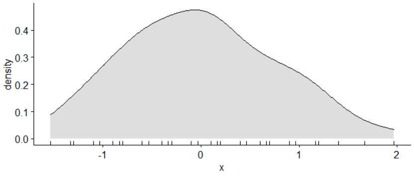
ggdensity(residuals, fill = "grey", rug = TRUE)

Density plot of model residuals

shapiro_test(residuals)

Shapiro test of model residuals

rstatix::levene_test(y ~ group, data = mydata)

Levene's test

lmtest::bptest(model_anova)

studentized Breusch-Pagan test

$\endgroup$
7
  • $\begingroup$ What are you measuring? What is your dependent variable? $\endgroup$
    – Stefan
    Commented Aug 31, 2020 at 12:53
  • $\begingroup$ I'm a genetics student so it's a biological effect that I've measured in a laboratory. It's sum of genotoxicity. Each row is a different unit of observation and sum of genotoxicity was calculated by adding 5 particular genetic aberrations that were observed in a single unit. Values are multiples of 0.5 because one genetic aberration is calculated in this way: 1/2000*1000 = 0.5, where 1 being the number of aberrant cells, 2000 total amount of observed cells, 1000 to get a promille. If you need more information I can get more into details. $\endgroup$
    – SamStark
    Commented Aug 31, 2020 at 17:06
  • $\begingroup$ Thanks for the detail, which I understand to imply that response values fall in [0, 5]. $\endgroup$
    – Nick Cox
    Commented Aug 31, 2020 at 17:27
  • $\begingroup$ Yes, exactly that. The upper limit in theory could go higher but biologicaly it's very unlikely with the conditions we used. Also, if I could ask one more question, do you think changing the total amount of observed cells would make sense from statistics point of view? In my lab it is common practice to just observe 2000 cells each time but I was thinking that maybe I could do 2100 cells one time, then 1900, then again 2000 my data wouldn't change that much but instead of 0.5 each time I could have 0.48 or 0.53. Would that make sense? $\endgroup$
    – SamStark
    Commented Sep 1, 2020 at 6:59
  • $\begingroup$ Slow to get it: your data are better analysed as a GLM with binomial family. Not being able to get 0.48 or whatever is secondary. The data really are 0, 1, ..., 10, .... in 2000. The normal as reference is not the best way to think about this at all. $\endgroup$
    – Nick Cox
    Commented Sep 1, 2020 at 7:33

1 Answer 1

3
$\begingroup$

Thanks for showing the data, but until the whole world uses R, your use of R syntax will be at best awkward and at worst not as helpful as you hope for those who don't use R. So for those people here is another listing of the your data.

y  group
1.5 "C"
  0 "C"
  1 "C"
  1 "C"
  1 "C"
  1 "C"
  1 "C"
  1 "C"
 .5 "C"
1.5 "C"
 .5 "C"
  1 "C"
 .5 "C"
  1 "C"
  1 "C"
 .5 "C"
  1 "C"
  2 "C"
 .5 "C"
2.5 "C"
1.5 "C"
  0 "C"
  1 "C"
  0 "C"
  2 "C"
 .5 "C"
 .5 "C"
1.5 "C"
  1 "C"
  2 "C"
 .5 "P"
  1 "P"
  2 "P"
2.5 "P"
1.5 "P"
  0 "P"
  2 "P"
  1 "P"
1.5 "P"
2.5 "P"
1.5 "P"
 .5 "P"
  1 "P"
3.5 "P"
  2 "P"
2.5 "P"
  3 "P"
  1 "P"
  3 "P"
3.5 "P"
1.5 "P"
  4 "P"
1.5 "P"
2.5 "P"
3.5 "P"
  1 "P"
  2 "P"
  2 "P"
  2 "P"
  2 "P"
2.5 "P"
  1 "P"
2.5 "P"
  1 "P"
  2 "P"
 .5 "P"
  2 "P"
2.5 "P"
  0 "P"
 .5 "P"
1.5 "P"
 .5 "P"
1.5 "P"
  1 "P"
 .5 "P"

and indeed that may not be convenient for everyone.

This normal quantile plot tells almost the whole story that we can discern.
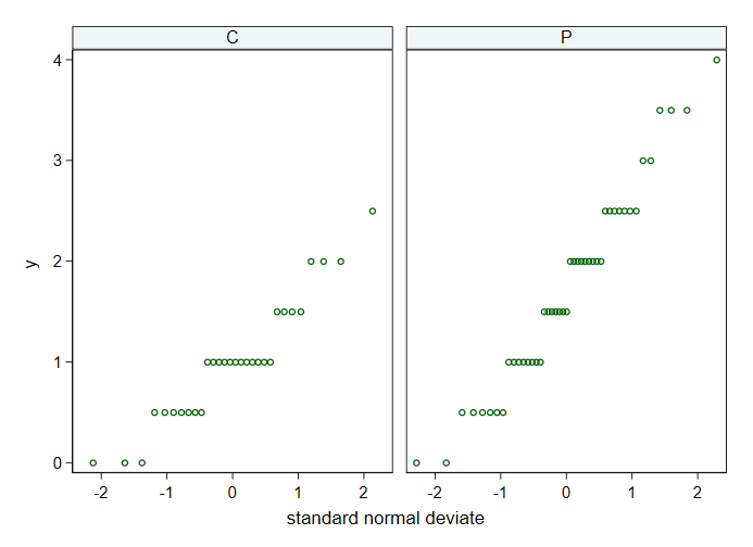
enter image description here

Sure, there is some slight skewness and heteroscedasticity visible there to the experienced eye, but neither is a big deal. And any idea that normal distributions are the goal here is compromised by the rounding of values as multiples of 0.5. Other way round, that requires flagging and some discussion. More: it seems a fair guess that your outcome cannot be negative and even that there may be an upper limit too: such a bound or bounds is also problematic for the ideal of a normal distribution.

In practice, a $t$ test whether using equal or unequal variances or a regression that ignores or respects heteroscedasticity all give unequivocal results, a convincing difference between the groups on this outcome. I show Stata results below and am confident that R code exists for the equivalent.

I disagree with your supervisor here. There is some departure from ideal assumptions but it is at worst a distraction. There is no need for, and no likely gain from, a transformation. I write as someone highly positive about using transformations -- when they really are needed and helpful.

. moments y , by(group)

----------------------------------------------------------------------
    Group |          n        mean          SD    skewness    kurtosis
----------+-----------------------------------------------------------
        C |         30       1.000       0.616       0.450       2.913
        P |         45       1.722       0.980       0.295       2.467
----------------------------------------------------------------------

. encode g, gen(Group)

. regress y i.Group

      Source |       SS           df       MS      Number of obs   =        75
-------------+----------------------------------   F(1, 73)        =     12.86
       Model |  9.38888889         1  9.38888889   Prob > F        =    0.0006
    Residual |  53.2777778        73  .729832572   R-squared       =    0.1498
-------------+----------------------------------   Adj R-squared   =    0.1382
       Total |  62.6666667        74  .846846847   Root MSE        =     .8543

------------------------------------------------------------------------------
           y |      Coef.   Std. Err.      t    P>|t|     [95% Conf. Interval]
-------------+----------------------------------------------------------------
       Group |
          P  |   .7222222    .201361     3.59   0.001     .3209103    1.123534
       _cons |          1   .1559736     6.41   0.000     .6891451    1.310855
------------------------------------------------------------------------------

. regress y i.Group, robust

Linear regression                               Number of obs     =         75
                                                F(1, 73)          =      15.34
                                                Prob > F          =     0.0002
                                                R-squared         =     0.1498
                                                Root MSE          =      .8543

------------------------------------------------------------------------------
             |               Robust
           y |      Coef.   Std. Err.      t    P>|t|     [95% Conf. Interval]
-------------+----------------------------------------------------------------
       Group |
          P  |   .7222222   .1844098     3.92   0.000     .3546939    1.089751
       _cons |          1   .1120584     8.92   0.000      .776668    1.223332
------------------------------------------------------------------------------

. ttest y, by(group)

Two-sample t test with equal variances
------------------------------------------------------------------------------
   Group |     Obs        Mean    Std. Err.   Std. Dev.   [95% Conf. Interval]
---------+--------------------------------------------------------------------
       C |      30           1    .1124441    .6158818     .770026    1.229974
       P |      45    1.722222    .1461246    .9802339    1.427727    2.016717
---------+--------------------------------------------------------------------
combined |      75    1.433333    .1062605    .9202428    1.221605    1.645062
---------+--------------------------------------------------------------------
    diff |           -.7222222     .201361               -1.123534   -.3209103
------------------------------------------------------------------------------
    diff = mean(C) - mean(P)                                      t =  -3.5867
Ho: diff = 0                                     degrees of freedom =       73

    Ha: diff < 0                 Ha: diff != 0                 Ha: diff > 0
 Pr(T < t) = 0.0003         Pr(|T| > |t|) = 0.0006          Pr(T > t) = 0.9997

. ttest y, by(group) unequal

Two-sample t test with unequal variances
------------------------------------------------------------------------------
   Group |     Obs        Mean    Std. Err.   Std. Dev.   [95% Conf. Interval]
---------+--------------------------------------------------------------------
       C |      30           1    .1124441    .6158818     .770026    1.229974
       P |      45    1.722222    .1461246    .9802339    1.427727    2.016717
---------+--------------------------------------------------------------------
combined |      75    1.433333    .1062605    .9202428    1.221605    1.645062
---------+--------------------------------------------------------------------
    diff |           -.7222222    .1843803               -1.089708   -.3547362
------------------------------------------------------------------------------
    diff = mean(C) - mean(P)                                      t =  -3.9170
Ho: diff = 0                     Satterthwaite's degrees of freedom =  72.8047

    Ha: diff < 0                 Ha: diff != 0                 Ha: diff > 0
 Pr(T < t) = 0.0001         Pr(|T| > |t|) = 0.0002          Pr(T > t) = 0.9999

Cautions and extra comments: I've noticed that some economists, and some other groups, are extraordinarily diligent at following a ritual that every ideal in sight is tested for formally. But for example Shapiro-Wilk here just shows that your sample size is big enough for departure from exact normality to be detectable -- and part of that departure is the discreteness (and boundedness?) that makes the assumption or ideal condition of normality a dubious goal in any case. A normal quantile plot is always a good idea too. The point of a normal quantile plot is not so much that normality is really important but rather that you are showing distributions in a standardised way and other kinds of behaviour will be evident too.

I would rather see a normal quantile plot of residuals if I have to choose just one graph to check on their distribution.

The advice you quote from McDonald is perhaps a little more optimistic than is justified, but I think it's more nearly pointing in the right direction.

EDIT: Much of that needs rewriting. The problem morphed in comments into a quite different one: comparing binomial distributions with small numerators and denominator 2000.

$\endgroup$
6
  • $\begingroup$ Thank you so much for such an insightful reply! I will keep in mind the listing of my data next time (I added your suggested format at the bottom of the post. Sorry for inconveniences). I just wanted to point out that there are actually five groups and not two but I get the idea of what you are saying. Also, I guess McDonald was referring to biological statistics in particular because of the nature of biological variance. I'm just more competent in my biological field but I'm really trying to learn statistics. Thanks again!!! $\endgroup$
    – SamStark
    Commented Aug 31, 2020 at 16:50
  • $\begingroup$ Thanks! I don’t regard biological statistics as fundamentally different from any other kind. What McDonald may say about that I don’t know. $\endgroup$
    – Nick Cox
    Commented Aug 31, 2020 at 17:31
  • $\begingroup$ Because parametric models are highly Y-transformation-dependent and because trying different transformations distorts standard errors of final parameter estimates, it is IMHO generally better to use a semiparametric regression model such as the proportional odds model, with no binning of Y. A detailed case study using ordinal models for a continuous outcome Y may be found in the RMS course notes. $\endgroup$ Commented Jan 15, 2022 at 15:37
  • $\begingroup$ @Frank Harrell How does that lead to different conclusions with the data example here? $\endgroup$
    – Nick Cox
    Commented Jan 15, 2022 at 16:13
  • $\begingroup$ Nick we don't know until we try it, but just on general principles semiparametric models are very efficient and it's a relief to not have to do a complicated bootstrap adjustment for model uncertainty when multiple models are entertained - jstor.org/stable/1390717 $\endgroup$ Commented Jan 15, 2022 at 17:45

Your Answer

By clicking “Post Your Answer”, you agree to our terms of service and acknowledge you have read our privacy policy.

Not the answer you're looking for? Browse other questions tagged or ask your own question.