Densities of Arrival Times of Poisson Process

Question

People arrive at a store as a non-homogeneous Poisson process with rate t, where t is the time measured in hours between noon and 6pm.

1. If we know that precisely one person arrived in the first hour, what is the density of its arrival time?

2. If we know that precisely two people arrived in the first hour, what is the density of the arrival time of the taller person? (height and arrival time are uncorrelated)

3. If we know that precisely two people arrived in the first hour, what is the density function of the arrival time of the person who arrived first?

4. If we know that at least one person arrived in the first hour, what is the density of the arrival time of the person who arrived first?

5. Assume that each person independently buys a geometric number of items with mean 2. What is the mean and variance of number of items sold before 2pm?

I am given from Campbell's Theorem that:

Let $S_n$ be the event times for a Poisson process. If $N_t=n$ is given then the vector $(S_1,s_2,\ldots,S_n)$ follows the distribution of ordered independent uniform variables $(U_{(1)},U_{(2)},\ldots,U_{(n)})$, where $U_i$ for $i=1,2,\ldots,n$ are independent uniform random variables on $[0,t]$, and $U_{(1)}$ is the minimum of $U_i$s, $U_{(2)}$ is the second smallest element, and so on. Consequently, the unordered set of arrival times $\left\{ S_1,\ldots,S_n\right\}$ has the same distribution $\left\{ U_1,\ldots,U_n\right\}$.

I'm fairly certain that for 1. and 2. they are both uniform on $(0,1)$, since for 2. we know that the $U_1$ and $U_2$ are independent from each other and that height and arrival time are uncorrelated, and 1. should follow quite simply from the theorem.

For 3. and 4. I'm unsure what to do. Starting with 3., would I be trying to find the density of $min\left\{U_1,U_2\right\}$? Then following for 4. that I'm asked to find the density of $min\left\{U_1,\ldots, U_n\right\}$? So do I need to find the cdf of the minimum and differentiate it, or am I going about this wrong.

For 5. since we have that the mean is $2$, then the number of items people by is $Geom(1/2)$. So I can quite simply work out the expected number of people arriving before 2pm and the mean will be $1/2$ multiplied by that expected value. However I have no clue how to calculate the variance.

Any help is greatly appreciated.

EDIT:

For 3., using some reference from this post: https://math.stackexchange.com/questions/1701172/conditional-probability-density-of-arrival-times

I worked out:

$$\begin{aligned} P(S_1\le s | N_1=2)&=\frac{P(S_1\le s, \; N_1=2)}{P(N_1=2)}\\ &=\frac{P(N_s=1, \; N_1-N_s=1)}{P(N_1=2)}\\ &=\frac{P(N_s=1) \;P(N_1-N_s=1)}{P(N_1=2)} \end{aligned}$$ $$N_s \;\text{is a Poisson}\;\left(\Lambda(s)= \int_0^st\;dt=\left.\frac{t^2}{2}\right|_{0}^{s}= \frac{s^2}{2} \right)\;\text{random variable}$$ $$P(N_s=1)=\frac{(s^2/2)^1 e^{-s^2/2}}{1!}=\frac{s^2}{2}e^{-s^2/2}$$ $$N_1-N_s \;\text{is a Poisson}\;\left(\Lambda(1)-\Lambda(s)= \int_s^1t\;dt=\left.\frac{t^2}{2}\right|_{s}^{1}= \frac{1}{2}-\frac{s^2}{2}=\frac{1-s^2}{2} \right)\;\text{random variable}$$ $$P(N_1-N_s=1)=\frac{((1-s^2)/2)^1e^{-(1-s^2)/2}}{1!}=\frac{1-s^2}{2}e^{(s^2-1)/2}$$ $$P(N_1=2)=\frac{(1/2)^2e^{-1/2}}{2!}=\frac{1}{8}e^{-1/2}$$ So, $$\begin{aligned} P(S_1\le s | N_1=2)&=\frac{P(N_s=1) \;P(N_1-N_s=1)}{P(N_1=2)}\\ &=\frac{\frac{s^2}{2}e^{-s^2/2}\cdot \frac{1-s^2}{2}e^{(s^2-1)/2}}{\frac{1}{8}e^{-1/2}}\\ &=\frac{\frac{s^2-s^4}{4}e^{-1/2}}{\frac{1}{8}e^{-1/2}}\\ &=2s^2-2s^4 \quad \text{, which is the cdf of }S_1 \text{ given that }N_1=2 \end{aligned} $$

But differentiating wrt $s$, I get that the pdf is $4s-8s^3$, which is not non-negative on the interval $(0,1)$. Where did I go wrong?

Answer 1

Computational

Question 5 is similarly based on different reason

It may often help to play a bit with some simple computations to get an idea how these arrivals look like.

Below I am using the method from the question What distribution to use to model time before a train arrives? to model the waiting time of arrivals as:

$$\begin{array}{} P(T_{\text{waiting time}} \leq t|T_{\text{waiting time}}>t_b) &=& 1- e^{-\int_{t_b}^t s(\tau) d\tau } \\&=& 1- e^{-\int_{t_b}^t \tau d\tau } \\&=& 1- e^{-0.5(t^2-t_b^2)}\end{array} $$

This gives the probability that the time will be $t$ or less, given the condition that we are starting to wait from $t_b$.

In the following code, we model these waiting times repeatedly and see how the distribution is:

### Function to sample waiting time
### We sample a quantile from a uniform distribution
### and compute it to a time based on the survival function
wait <- function(t) {
  qs <- exp(-0.5*t^2)
  q <- runif(1,0,qs) ### sample quantile from uniform distribution
  t_out <- sqrt(-2*log(q))
  return(t_out)
}

### simulate the process n times
n = 5000
set.seed(1)
tt = c() ### this variable will contain all the simulated times
t1 = c() ### this variable will contain times when only 1 customer got in during the 1st hour
t2 = c() ### this variable will contain times when 2 customer got in during the 1st hour

for (i in 1:n) {
  t <- wait(0)
  ### keep sampling customers while the time is below 6 hours
  while (tail(t,1)<6) {
    t <- c(t,wait(tail(t,1)))
  }
  
  ### store the times 't' into a larger variable 'tt' for plotting histogram
  ## we do this by appaneding it to the current 'tt'
  tt <- c(tt,t[t<6])
  
  ### Store time if precisely one person arrived in the first hour
  if ( sum(t<1) == 1 )  {
    t1 <- c(t1,t[1])
  }

  ### Store time if precisely two persons arrived in the first hour
  if ( sum(t<1) == 2 )  {
    t2 <- c(t2,t[1])
  }
}

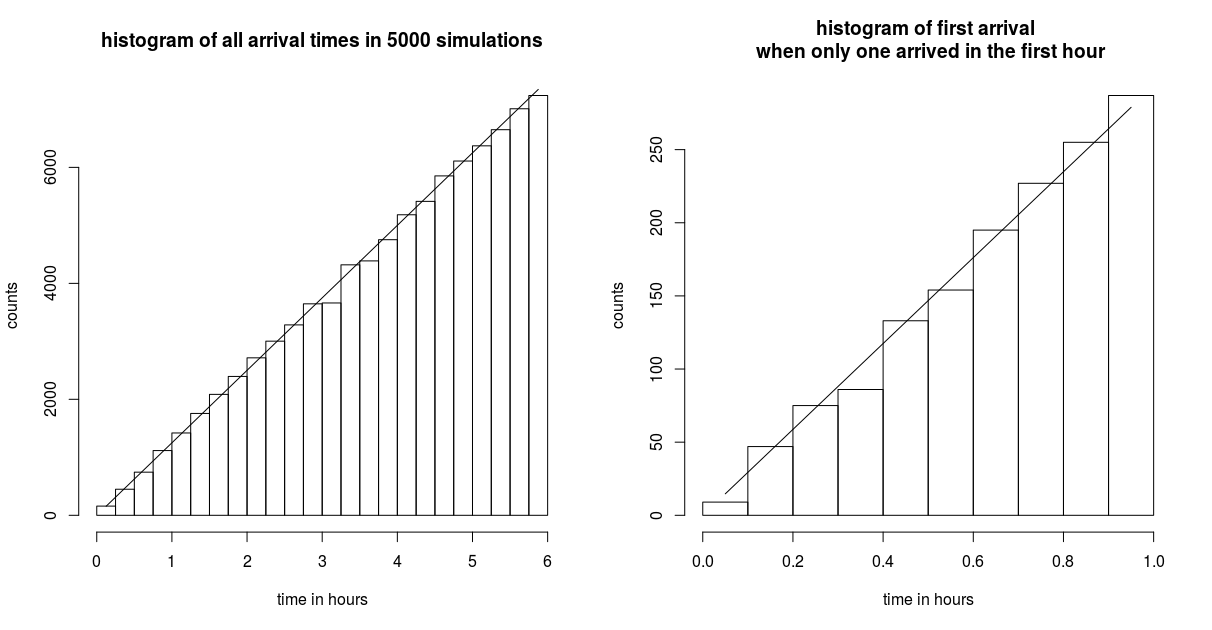
### histogram of all cases
h <- hist(tt, breaks = seq(0,6,0.25))
lines(h$mids,h$mids*n*0.25)

### histogram of first arrival when only one arrived in the first hour
h <- hist(t1, breaks =seq(0,1,0.1))
lines(h$mids,h$mids*2*length(t1)*0.1)


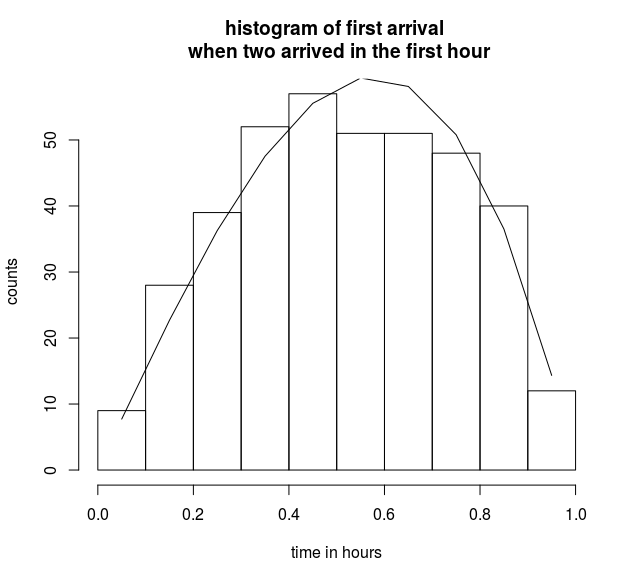
### histogram of first arrival when exactly two arrived in the first hour
h <- hist(t2, breaks =seq(0,1,0.1), main = "histogram of first arrival \n when two arrived in the first hour", xlab = "time in hours",
          ylab = "counts")
lines(h$mids,2*(2-2*h$mids^2)*h$mids *length(t2)*0.1)

It is no surprise that the distribution of times is equal to a linear function of time since we considered "a non-homogeneous Poisson process with rate t".

But in the histogram on the right, we see that the same is true for the distribution of arrival times when we look at the time of the first arrival time, conditional on only one arrival in the first hour.

Inuition behind Campbell's theorem

The derivation below is a bit handwavy, viewing the density as a probability for time $t$ to $t+dt$. I personally find this more intuitive. If you like a more rigorous derivation then you could follow the same logic and express the cumulative distribution and take the derivative of that cumulative distribution

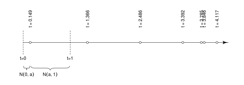
The example image below shows a simulation in which case there is only one arrival within the first hour.

We could express the number of arrivals:

• before the point $t_1$: the number of arrivals $N_{0,t_1}$ from the time $0$ and till time $t_1$
• after the point $t_1$: the number of arrivals $N_{t_1,1}$ from the time $t_1$ and till time $1$. In the example we have for $a=0.5$ the situation that $N_{0,a} = 1$ and $N_{a,1} = 0$.

In relation to the question

• "What is the density for the $n$-th arrival time, if the total arrivals is $m$?"

We can look at the question

• "What is the probability that there is an arrival from $t$ to $t+dt$ and there are $n-1$ arrivals before it and $m-n$ arrivals behind it?".

This density is the rate multiplied two Poisson distributed variables (for the probability of $n-1$ arrivals before and $m-n$ arrivals behind the arrival that is being considered) and divided by a Poisson distributed variable (the probability to have $m$ arrivals) as a normalization:

$$\begin{array}{} f(t;n,m) &=& s(t) \frac{P(N_{0,t} = n-1) P(N_{t,1} = m-n)}{P(N_{0,1} = m)} \\ &=& s(t) \frac{\frac{\lambda_1^{n-1} e^{-\lambda_1}}{(n-1)!} \frac{\lambda_2^{m-n} e^{-\lambda_2}}{(m-n)!}}{\frac{\lambda_3^{m} e^{-\lambda_3}}{(m)!}} \\ & =& s(t) \frac{m!}{(m-n)!(n-1)!} \frac{\lambda_1^{n-1}\lambda_2^{m-n}}{\lambda_3^{m}} \end{array}$$

And these $\lambda_i$ relate to the rates for the number of arrivals in the specific time frame which are the integrals of, $s(t)$, the rate of arrivals as function of time, $\lambda_1 = \int_{0}^{t} s(u) du$, $\lambda_2 = \int_{t}^{1} s(u) dt$ and $\lambda_3 = \int_{0}^{1} s(u) du$.

When we view $g(t) = s(t)/\int_{0}^{1} s(t) dt$ as a probability density function and $G(t)$ the cumulative distribution function then the above turns into

$f(t;n,m) = s(t) \frac{m!}{(m-n)!(n-1)!} \frac{\left( \int_{0}^{t} s(u) dt\right)^{n-1}\left( \int_{t}^{1} s(u) dt\right)^{m-n}}{\left( \int_{0}^{1} s(u) dt\right)^{m}} = g(t) G(t)^{n-1} (1-G(t))^{m-n} $

This relates to the function of the order statistic, and also has a similar description/derivation here.

Using Campbell's theorem

If we know that precisely two people arrived in the first hour, what is the density function of the arrival time of the person who arrived first?

To compute an order statistic you can use some sort of inverse transform sampling and describe the order statistic of the quantile which is a uniform distribution (if the underlying distribution is continuous) and this follows the beta distribution (see also here).

So the for the 1-st order statistic for a sample of size 2 the quantile will be distributed as $Beta(1,2)$:

$$f_Q(q) = 2-2q \quad \text{for $0\leq q \leq 1$}$$

And we have (with $s(\tau) = \tau$) the following transformation between the time $t$ of the arrival and the quantile of it's distribution

$$q = \frac {\int_0^t s(\tau) d\tau}{ {\int_0^1 s(\tau) d\tau}} = t^2$$

The distribution of $t$ is found by transforming the distribution of $q$

$$f_T(t) = f_Q(t^2) \frac{\partial q}{\partial t} = 4t-4 t^3 \quad \text{for $0\leq t \leq 1$}$$

This solution does match the simulations

Your computation is very similar but has a factor $8$ in place of $4$.

I guess that you will get the same when you use

$$\begin{aligned}{} P(S_1\le s | N_1=2)&=\frac{P(S_1\le s, \; N_1=2)}{P(N_1=2)}\\ &=\frac{P(N_s=1, \; N_1-N_s=1) + P(N_s=2, \; N_1-N_s=0)}{P(N_1=2)}\\ &=\frac{P(N_s=1) \;P(N_1-N_s=1) + P(N_s=2) \;P(N_1-N_s=0)}{P(N_1=2)} \end{aligned}$$

The other questions

For question 1 you can use Campbell's theorem but it is not really necessary.

For question 2, 4 and 5 you need to use different reasoning. These questions are not about the order.