7
$\begingroup$

The likelihood function is not in general a PDF (there have been many questions on this). e.g. if we take the binomial likelihood, $$P(Evidence \mid \theta) = f(\theta) = {n \choose k} \theta^k (1-\theta)^{n-k}$$ it does not integrate to 1. In general (and say, for $n=2$ and $k=3$): $$\int_{0}^1 f(\theta) d\theta \neq 1$$

But I believe in some cases, the likelihood does integrate to 1. For example, if the likelihood function is a normal PDF, like in the case of a normal-normal conjugate prior setup. Then $$P(Evidence \mid \theta)=f(\theta)=NormalPDF_{\mu,\sigma}(\theta)$$ and $$\int_{\mathbb{R}} f(\theta)d\theta = 1$$.

Is there an intuitive explanation for the fact that this particular likelihood function is a PDF?. Even better, can someone give insightful necessary and sufficient conditions for a likelihood function being a PDF?

$\endgroup$
5
  • $\begingroup$ @Xi'an: Not sure I understand your concern accurately. If a think of a concrete example where $\Theta$ is say the effect of a medicine on a disease, it seems there is a natural measure over that? $\endgroup$
    – tmkadamcz
    Commented Dec 12, 2020 at 22:07
  • $\begingroup$ What would the natural measure be on a probability $p$? on an odd-ratio $p/(1-p)$? on its logit transform $\log\{p/(1-p)\}$? $\endgroup$
    – Xi'an
    Commented Dec 13, 2020 at 9:27
  • 2
    $\begingroup$ Your binomial expression is only proportional to likelihood (and it is usual to have $n \ge k$). For example you might drop the ${n \choose k}$ element if you knew the outcomes in order, but knowing this order should not affect any inference. So the likelihood integrating to $1$ over a parameter is a coincidence (and possibly an arithmetic convenience if you can spot this without having to do the integration). $\endgroup$
    – Henry
    Commented Dec 14, 2020 at 10:18
  • $\begingroup$ @Henry: good comment about the ambiguity of handling the likelihood as the full data density versus a sufficient statistic density. $\endgroup$
    – Xi'an
    Commented Dec 14, 2020 at 15:24
  • 1
    $\begingroup$ @Xi'an sure thing, done. $\endgroup$
    – tmkadamcz
    Commented Dec 14, 2020 at 20:57

5 Answers 5

8
$\begingroup$

The purpose of this answer is to show that the situation is so rich and complicated that it's unlikely there exists any simple characterization of such distributional families.

I will first show, by construction, that there are many such families and they are flexible and varied. Then I will show that even this construction doesn't cover the gamut of possibilities. In this process, though, we might improve our intuition about what it means for the likelihood of a single real parameter to be a density function.


When $\theta$ can range over all the real numbers and is a location parameter -- that is, when the distribution functions are all of the form $f(x-\theta)$ for some density $f$ -- it is easy to see that integrating over the parameter $\theta$ gives the constant value $1.$

Let's play with this a little. What if, for instance, we were to take two distinct densities $f_1$ and $f_2$ and let $\theta$ play the role of a location parameter for each one of them, but in two different ways? For instance, form the family of functions

$$f(x,\theta) = a_1f_1(x-2\theta) + a_2f_2(x-\theta/2)$$

where the $a_i$ are to be determined. By simple substitutions $x=y+\theta$ and $x=y+\theta/2,$ compute that

$$\begin{aligned} \int_{\mathbb{R}}f(x,\theta)\,\mathrm{d}x &= \int_{\mathbb{R}}a_1f_1(x-2\theta)\,\mathrm{d}x + \int_{\mathbb{R}}a_2f_2(x-\theta/2)\,\mathrm{d}x\\ &= a_1\int_{\mathbb{R}}f_1(y)\,\mathrm{d}y + a_2\int_{\mathbb{R}}f_2(y)\,\mathrm{d}y\\ &= a_1+a_2. \end{aligned}$$

Thus, provided $a_1+a_2 = 1$ and $f(x,\theta)\ge 0$ for all $x,$ $x\to f(x,\theta)$ is a probability density. When we integrate over the parameter $\theta$ we obtain, using the same methods of substituting $\theta=(y+x)/2$ and $\theta=2(y+x),$

$$\begin{aligned} \int_{\mathbb{R}}f(x,\theta)\,\mathrm{d}\theta &= \int_{\mathbb{R}}a_1f_1(x-2\theta)\,\mathrm{d}\theta + \int_{\mathbb{R}}a_2f_2(x-\theta/2)\,\mathrm{d}\theta \\ &= \frac{1}{2}a_1\int_{\mathbb{R}}f_1(y)\,\mathrm{d}y + 2a_2\int_{\mathbb{R}}f_2(y)\,\mathrm{d}y\\ &= \frac{1}{2}a_1+2a_2. \end{aligned}$$

By setting $a_1=2/3$ and $a_2=1/3$ we can make this result unity for all $x$ as well as guaranteeing $f$ has no negative values, thereby satisfying the conditions of the problem. With some care we can also make this family of distributions identifiable in the sense that each $\theta$ determines a unique distribution, as I will show by example. However, $\theta$ is not a location parameter.

An example illustrates why not. Let $f_2$ be the Uniform$[0,1]$ density and $f_1$ be a Normal density with variance $1/3$ and mean $0.$ Here are some plots of $f$ for various values of $\theta:$

Figure

As $\theta$ increases (from left to right), the rectangular part of the density (the Uniform component) marches slowly rightward while the curved part of the density (the Normal component) marches rightward four times faster. The resulting distributions are all obviously different. Effectively, $\theta$ does determine a "location" of sorts, but it also determines the shape of the distribution. That's why it's not a location parameter.

This construction can be vastly generalized to create rich, flexible families of distributions having all the properties in the question but (in general) not being location families. For completeness, I will give the details before proceeding with the main question.

Let $f:\mathbb{R}\times\mathbb{R}\to[0,\infty)$ be any integrable family of distribution functions; that is, for all numbers $\lambda$

$$\int_{\mathbb{R}}f(x,\lambda)\,\mathrm{d}x = 1.$$

Consider any distribution function $G$ supported on the nonnegative real numbers and use it to form the family $\mathcal G$ of functions $g:\mathbb{R}\times\mathbb{R}\to[0,\infty)$ via

$$g(x,\theta) = \int_0^\infty f\left(x - \frac{\theta}{\lambda}\right)\,\mathrm{d}G(\lambda).$$

For each $\theta$ this gives a density function because obviously $g(x,\theta)\ge 0$ and

$$\begin{aligned} \int_\mathbb{R}g(x,\theta)\,\mathrm{d}x &= \int_\mathbb{R}\int_0^\infty f\left(x - \frac{\theta}{\lambda}\right)\,\mathrm{d}G(\lambda)\,\mathrm{d}x\\ &= \int_0^\infty \int_\mathbb{R}f\left(x - \frac{\theta}{\lambda}\right)\,\mathrm{d}x\,\mathrm{d}G(\lambda)\\ &= \int_0^\infty (1)\,\mathrm{d}G(\lambda)\\ &= 1. \end{aligned}$$

Integrating instead over $\theta$ using the substitution $\theta=y\lambda$ yields

$$\begin{aligned} \int_\mathbb{R}g(x,\theta)\,\mathrm{d}\theta&= \int_\mathbb{R}\int_0^\infty f\left(x - \frac{\theta}{\lambda}\right)\,\mathrm{d}G(\lambda)\,\mathrm{d}\theta\\ &= \int_0^\infty \int_\mathbb{R}f\left(x - \frac{\theta}{\lambda}\right)\,\mathrm{d}\theta\,\mathrm{d}G(\lambda)\\ &= \int_0^\infty \int_\mathbb{R}f\left(x - \frac{y\lambda}{\lambda}\right)\,\mathrm{d}\left(y\lambda\right)\,\mathrm{d}G(\lambda)\\ &= \int_0^\infty \int_\mathbb{R}f\left(x - y\right)\,\mathrm{d}y\,\lambda\,\mathrm{d}G(\lambda)\\ &= \int_0^\infty\lambda\,\mathrm{d}G(\lambda). \end{aligned}$$

If we further stipulate that the expectation of $G$ is unity, this shows that the family $\mathcal G$ satisfies the conditions of the question. However, except in special cases, $\theta$ is not a location parameter.


Let's consider the natural follow-up question: when the likelihood is a PDF in the sense of the question, can we always represent the family as a mixture in the foregoing sense?

Unfortunately the answer is no. As a counterexample, consider the family of distribution functions given by

$$f(x,\theta) = 2\left(\left\{\theta\right\} + \left(x - \lfloor \theta \rfloor\right) - 2 \left\{\theta\right\}\left(x - \lfloor \theta \rfloor\right)\right)$$

where $\lfloor \theta \rfloor$ is the greatest integer less than or equal to $\theta$ and $\left\{\theta\right\} = \theta - \lfloor \theta \rfloor$ is the fractional part of $\theta$ (lying in the interval $[0,1)$).

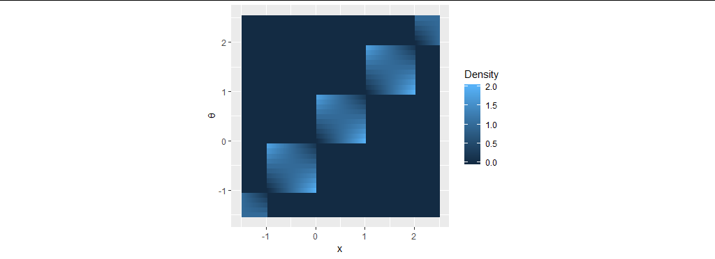
This strange looking function describes distributions defined on intervals $[n,n+1)$ (where $n = \lfloor \theta \rfloor$) that vary according to the fractional part of $\theta.$ Here are some of their densities:

Figure 2

Here is a plot of $f:$

Figure 3

Now if this family had a location parameter $\mu = \mu(\theta),$ we would be able to express each $f(x,\theta)$ as a fixed function of $x-\mu(\theta).$ Its level sets (contours) would therefore be unions of lines of the form $x-\mu=\text{constant};$ that is, of lines with 45 degree slopes. Geometrically, this means we can stretch and compress this image purely in the vertical ($\theta$) direction until its bright patches--where the density is nonzero--become a slanted band with parallel linear contours.

No matter how we might re-express the parameter $\theta$ (in a continuous fashion), obviously there's no way it can change this checkered pattern into such an image.

$\endgroup$
4
  • 1
    $\begingroup$ Just to add one stone to this beautiful construction of an answer, the very first issue is that the likelihood function is constructed in the absence of a measure $\text d\mu(\theta)$ over the parameter space. Since there is no "natural" construction for the said measure, the question is somehow moot. $\endgroup$
    – Xi'an
    Commented Dec 12, 2020 at 17:53
  • 1
    $\begingroup$ @Xi'an (Thank you.) I had a similar feeling initially, but kept coming back to this question because of a nagging feeling there is something intrinsic about Lebesgue measure here: it is the invariant measure under the affine group. With that in mind, it's possible to formulate analogs of this situation for other groups (such as the multiplicative group). Consequently, I don't think I am as prepared as you are to dismiss this altogether. $\endgroup$
    – whuber
    Commented Dec 12, 2020 at 21:21
  • $\begingroup$ Thank you, this is very thorough. Even just the sufficient condition you gave at the start of the answer was helpful. $\endgroup$
    – tmkadamcz
    Commented Dec 12, 2020 at 22:18
  • $\begingroup$ If it matters for the problem at hand, invariance is a form of prior information (but there are others, possibly conflicting) and group actions leading to a unique right Haar measure are quite rare. The simplest counter-example is the Poisson model. $\endgroup$
    – Xi'an
    Commented Dec 13, 2020 at 9:41
4
$\begingroup$

There is a similar question here: What is the reason that a likelihood function is not a pdf?

Hopefully, that can be of help. In particular see whuber's comment regarding Fishers 1922 article:

Integrating to unity is beside the point. Fisher, in a 1922 paper On the Mathematical Foundations of Theoretical Statistics, observed that indeed usually the likelihood L(θ) can be "normalized" to integrate to unity upon multiplying by a suitable function p(θ) so that ∫L(θ)p(θ)dθ=1. What he objected to is the arbitrariness: there are many p that work. "...the word probability is wrongly used in such a connection: probability is a ratio of frequencies, and about the frequencies of such values we can know nothing whatever."

It seems that this indicates that there would exist an arbitrary number of likelihood functions that post normalization would be integratable to 1.

Then the distinction would seem to lie in the fact that a likelihood function is a measure of goodness of fit. Thus, if we look at a graph of a likelihood function a point is the likelihood of a parameter $\theta$ for a given observed outcome.

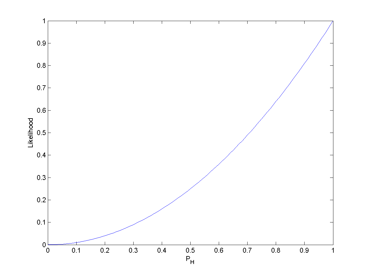
enter image description here

In the image above: is the likelihood function of $p_(H)^2$ the probability of a coin landing heads up (without prior knowledge) given we have observed HH. Where $P_H$ is $\theta$ the true probability of the coin landing heads. -https://en.wikipedia.org/wiki/Likelihood_function

In the case of a PDF any "any given sample (or point) in the sample space (the set of possible values taken by the random variable) can be interpreted as providing a relative likelihood that the value of the random variable would equal that sample."- https://en.wikipedia.org/wiki/Probability_density_function Where, as I see it, the sample would have fixed parameters.

to summarize, a likelihood function gives probability of a parameter for an observed outcome. Where as pdf gives likelihood that a random variable belongs to the sample.

Hopefully someone that knows more can chime in and answer your question directly

$\endgroup$
4
  • $\begingroup$ Very good point, esp. recalling Fisher's 1922 objection! $\endgroup$
    – Xi'an
    Commented Dec 12, 2020 at 18:22
  • 1
    $\begingroup$ Multiplying the likelihood with a function $p(\theta)$ is more like equivalent to computing a posterior distribution. It is not normalizing the likelihood function because it changes the shape of the likelihood function. To normalize you would need to multiply with a constant (constant as function of $\theta$ but it may vary as a function of the observations). There are an arbitrary number of posterior functions bit there is only a single way to normalize the likelihood function. $\endgroup$ Commented Dec 12, 2020 at 19:50
  • $\begingroup$ The problem is instead that normalizing the likelihood function to integrate to 1 does not yet make it a function that can be interpreted as a probability density. (For a function that can be interpreted as a probability you'd need to compute the fiducial distribution which is like the likelihood but not the same). $\endgroup$ Commented Dec 12, 2020 at 19:53
  • $\begingroup$ (i) Whatever dominating measure $\text d\lambda$ one picks, it multiplies the likelihood by this measure, this cannot be avoided when turning the likelihood into a probability density. (ii) There is one way to normalize the likelihood per dominating measure. (iii) The seemingly natural $\text d\theta$ does not stand a change of parameterisation: if $\theta=h(\eta)$, the transformed measure is $|h'(\eta)|\text d\eta$, not $d\eta$. $\endgroup$
    – Xi'an
    Commented Dec 13, 2020 at 9:47
3
$\begingroup$

The mean of a normal distribution is a location parameter. In general, if $\theta$ is a location parameter, then:

$$\int_{\theta \in \mathbb{R}}g_{\theta}(x_0)\:d\theta = \int_{x \in \mathbb{R}}g_o(x_0 - x)\:dx = \int_{x \in \mathbb{R}}g_o(x)\:dx = 1$$

where $g_0$ is the pdf when $\theta = 0$.

$\endgroup$
1
$\begingroup$

To quote from Ronald Fisher himself (and intersecting with the answer by NicoFish as well as the answer by WHuber to the earlier question):

  1. when defining the likelihood function (as a function of the parameter $\theta$), Fisher (in his 1912 undergraduate memoir) warns against integrating it w.r.t. the parameter: “the integration with respect to [the mean parameter] $m$ is illegitimate and has no definite meaning with respect to inverse probability. [The likelihood is] a relative probability only, suitable to compare point with point, but incapable of being interpreted as a probability distribution over a region, or of giving any estimate of absolute probability.” And again in 1922: “[the likelihood] is not a differential element, and is incapable of being integrated: it is assigned to a particular point of the range of variation, not to a particular element of it”.
  2. He introduced the very term “likelihood” especially to avoid the confusion with a probability density and to separate it and himself from Bayesian analysis: “I perceive that the word probability is wrongly used in such a connection: probability is a ratio of frequencies, and about the frequencies of such values we can know nothing whatever (…) I suggest that we may speak without confusion of the likelihood of one value of $p$ being thrice the likelihood of another (…) likelihood is not here used loosely as a synonym of probability, but simply to express the relative frequencies with which such values of the hypothetical quantity $p$ would in fact yield the observed sample”. [Which I understand as a defense of the relativity of the likelihood values, which connects with the point that it is only defined up to a multiplicative constant, as e.g. when comparing the likelihood for the entire sample and for a sufficient statistic.]
  3. Another point he makes repeatedly (both in 1912 and 1922) is the lack of invariance of the probability measure obtained by attaching a d$θ$ to the likelihood function $L(θ)$ and normalising it into a density: while the likelihood “is entirely unchanged by any [one-to-one] transformation”, this definition of a probability distribution is not. Fisher actually distanced himself from a Bayesian “uniform prior” throughout the 1920’s and opting for a uniform (improper) prior is indeed making an arbitrary choice of a particular prior. [Which connects with my critical answer that to turn the likelihood into a density, a dominating measure must first be chosen and that there is no compelling argument to make the Lebesgue measure as a default choice.]

Fisher however made things more complicated when introducing the fiducial distribution in the 1950's since, to quote from Dennis Lindley (1958):

according to Fisher (1956) [the fact that the fiducial distribution is consistent under sequential updating] is true, though no formal proof is given, for he says (p. 51) "The concept of probability involved [in the fiducial argument] is entirely identical with the classical probability of the early writers, such as Bayes". Again he says (p. 125) "This fiducial distribution supplies information of exactly the same sort as would a distribution given a priori".

Although this is not exactly related with the original question, but for a uniform prior being used in both instances, let me point out that Lindley (1958) establishes that "therefore the fiducial argument is only consistent in the case of a single sufficient statistic when the distribution is of the gamma or normal forms, or transformable thereto."

$\endgroup$
0
$\begingroup$

The likelihood is not a PDF

Is there an intuitive explanation for the fact that this particular likelihood function is a PDF?

This is a loaded question. It is based on a wrong premise. The likelihood function is not a PDF.

The condition $\int_{\theta \in \mathbb{R}} f(\theta) d\theta= 1$ is a necessary condition for some function $f(\theta)$ to be a PDF but it is not a sufficient condition for the function to be a PDF.

For some function to be a PDF it must also have a probability interpretation. The likelihood function does not have this interpretation (not by itselve). Yes, the likelihood is the probability density of observing $x$, but as a function of $\theta$ it looses the interpretation of a probability density or mass function. The likelihood function is 'a function of probability densities' but it is not a probability density itselve.

A probability density is a function $f$ such that the integral over some differential measure $\theta$ on a set of events $\Omega$ gives a measure of the joint probability for those events in the set $P(\Omega) = \int_\omega f d\theta$

  • The quantity $\int_a^b f_X(x|\theta) dx$ is a probability (namely the frequency of events $a \leq x \leq b$)
  • But the quantity $\int_a^b \mathcal{L}(\theta|x) d\theta$ is not a probability. It has no probabilistic meaning.

Analogous example in physics: You may have a mass density that is a function of both space and temperature. The mass density as a function of temperature should not be interpreted as the density expressing the amount of mass per amount of temperature.

Likelihood's that sum up to 1

A likelihood can sum to 1 but if this is the case then this is a coincidence. This is not a special property for some cases. For any case you have a likelihood function that sums to 1.

Likelihood functions are defined as being proportional to the probability density or mass of $x$ as function of $\theta$ $$\mathcal{L}(\theta|x) = c \cdot f_X(x|\theta)$$ where $c$ can be any constant and there is always* some $c$ such that you can make the likelihood function integrate to 1.

*Possibly there might be some pathological case where there is some observation $x$ with infinite density such that $\int_{\theta \in \mathbb{R}} f(x|\theta) d\theta$ is infinite.

The likelihood function can be mathematically equivalent to a probability

  • The likelihood function (when properly normalized) coincides with the formula for a probability density if the prior distribution is uniform. In this case the likelihood function and the posterior probability density are equal. In this case you might say that the likelihood function has a probabilistic interpretation (Although it is just that the formula for the likelihood coincides with the formula for the posterior pdf; The concept of likelihood does not turn into a probability)

  • The likelihood function sometimes coincides with the fiducial distribution or confidence distribution. The fiducial density is similar to the likelihood but based on the CDF.

    $$\begin{array}{rrcl} \text{Likelihood: } & \mathcal{L}(\theta|x) &\propto& f_X(x|\theta)\\ \text{Fiducial distribution: } & \mathcal{F}(\theta|x) &= & F_X(x|\theta) \end{array}$$

    In this case it can also be considered to coincide with a probabilistic interpretation. (But it is not a probability in the typical sense. Similar to the confidence interval it does not relate to the probability for the parameter conditional on the observation)

$\endgroup$
3
  • $\begingroup$ Thanks for the answer. Not sure I understand about the likelihood function not having a probability interpretation. Isn't it simply the probability of observing the evidence $E$ given a value $\theta$ of $\Theta$, i.e. $P(E \mid \theta)$? $\endgroup$
    – tmkadamcz
    Commented Dec 12, 2020 at 22:11
  • $\begingroup$ @tmkadamcz Yes, it is the probability density of observing $E$, but as a function of $\theta$ it looses the interpretation of probability. $\endgroup$ Commented Dec 12, 2020 at 22:39
  • $\begingroup$ @tmkadamcz I have integrated my comment into the answer. What do you think of it? $\endgroup$ Commented Dec 13, 2020 at 10:43

Your Answer

By clicking “Post Your Answer”, you agree to our terms of service and acknowledge you have read our privacy policy.

Not the answer you're looking for? Browse other questions tagged or ask your own question.