Bayesian Prediction Simple Explanation

Question

I have read through other questions on the site and I feel that none provide a great answer to this question. Simply put - could anyone explain, common approaches for generating predictions on new unseen data with a Bayesian model.

For example, suppose you have a simple linear regression: $$ y = \alpha + \beta * x $$

Which under a probabilistic framework is given by:

$$ y \sim N(\mu = \alpha + \beta *x, \sigma = \epsilon) $$

We set prior distributions for the parameters $ \alpha, \beta$ and $\epsilon$ and with our training data $X_{train}$ we return samples from posterior to obtain posterior distributions across these parameters.

My question is, given new data $X_{new}$, how are predictions then made on that data?

For example, would you:

• For each new data point in $X_{new}$, take the posterior samples from the 'training' process, and calculate $Y_{new}$ using combinations of coefficients from the posterior samples (for a given data point in $X_{new}$) - to generate a vector of predictions for each data point in $X_{new}$?

Answer 1

Correct.

You have draws from posterior, so for a new $x_i$ the corresponding prediction for $\mu$ is $\dfrac{1}{N} \sum _i \alpha_i + \beta_i x%$. If you're familliar with rstanarm, this is what posterior_linpred does. Since the predictor is linear, this should be equal to $E(\alpha) + E(\beta)x$, where $E$ is the expectation. Here is an example using Stan.

Let's first set up the model and fit it.

library(tidyverse)
library(tidybayes)
library(cmdstanr)

model_code = '
data{
  int N;
  vector[N] x;
  vector[N] y;
}
parameters{
  real alpha;
  real beta;
  real<lower=0> sigma;
}
model{
  alpha ~ normal(0,1);
  beta ~ normal(0,1);
  sigma ~ cauchy(0,1);
  y ~ normal(alpha + beta*x, sigma);
}
generated quantities{
  real yppc[N] = normal_rng(alpha + beta*x, sigma);
}
'
fl = write_stan_file(model_code)
model = cmdstan_model(fl)

N = 10
x = rnorm(N)
y = 2*x + 1 + rnorm(N, 0, 0.45)
model_data = list(N=N, x=x, y=y)
fit = model$sample(model_data, parallel_chains=4)

Now, extract the draws

beta = as.numeric(fit$draws('beta'))
alpha = as.numeric(fit$draws('alpha'))
sigma = as.numeric(fit$draws('sigma'))

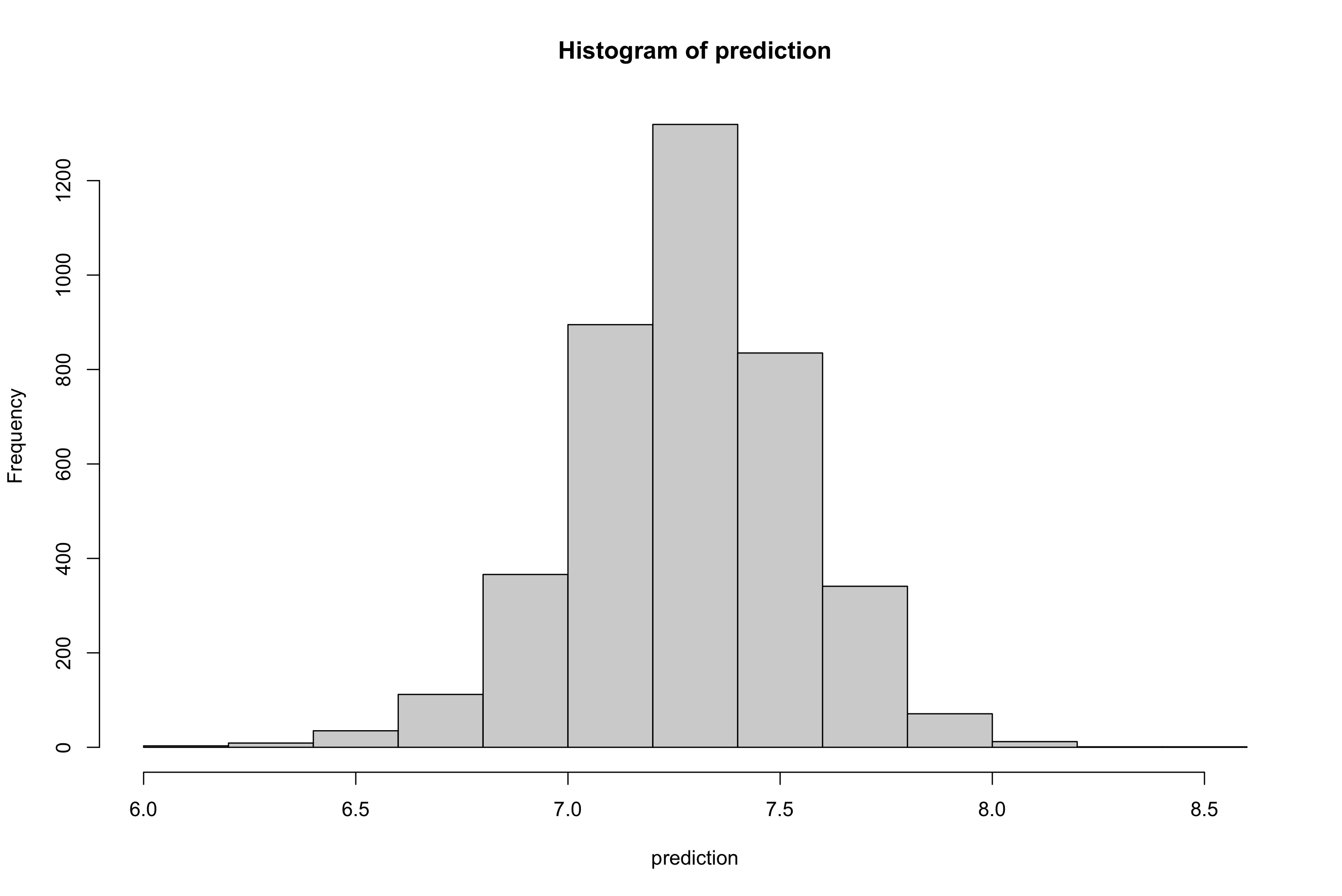
Let's say I want to make a prediction for $x=3$. I should compute $\alpha_i + \beta_i \cdot 3$ for all my posterior $\alpha_i, \beta_i$. In R...

prediction = alpha + beta*3
hist(prediction)

Note that we get a distribution of possible values. Our prediction in this case is the mean of this distribution

mean(prediction)
>>>7.281336

Which is close to the true value of 7.