Moment generating function of the inner product of two gaussian random vectors

Question

Can anybody please suggest how I can compute the moment generating function of the inner product of two Gaussian random vectors, each distributed as $\mathcal N(0,\sigma^2)$, independent of each other? Is there some standard result available for this? Any pointer is highly appreciated.

Answer 1

First let's address the case $\Sigma = \sigma\mathbb{I}$. At the end is the (easy) generalization to arbitrary $\Sigma$.

Begin by observing the inner product is the sum of iid variables, each of them the product of two independent Normal$(0,\sigma)$ variates, thereby reducing the question to finding the mgf of the latter, because the mgf of a sum is the product of the mgfs.

The mgf can be found by integration, but there's an easier way. When $X$ and $Y$ are standard normal,

$$XY = ((X+Y)/2)^2 - ((X-Y)/2)^2$$

is a difference of two independent scaled Chi-squared variates. (The scale factor is $1/2$ because the variances of $(X\pm Y)/2$ equal $1/2$.) Because the mgf of a chi-squared variate is $1/\sqrt{1 - 2\omega}$, the mgf of $((X+Y)/2)^2$ is $1/\sqrt{1-\omega}$ and the mgf of $-((X-Y)/2)^2$ is $1/\sqrt{1+\omega}$. Multiplying, we find that the desired mgf equals $1/\sqrt{1-\omega^2}$.

(For later reference, notice that when $X$ and $Y$ are rescaled by $\sigma$, their product scales by $\sigma^2$, whence $\omega$ should scale by $\sigma^2$, too.)

This should look familiar: up to some constant factors and a sign, it looks like the probability density for a Student t distribution with $0$ degrees of freedom. (Indeed, if we had been working with characteristic functions instead of mgfs, we would obtain $1/\sqrt{1 + \omega^2}$, which is even closer to a Student t PDF.) Never mind that there is no such thing as a Student t with $0$ dfs--all that matters is that the mgf be analytic in a neighborhood of $0$ and this clearly is (by the Binomial Theorem).

It follows immediately that the distribution of the inner product of these iid Gaussian $n$-vectors has mgf equal to the $n$-fold product of this mgf,

$$(1 - \omega^2 \sigma^4)^{-n/2}, \quad n=1, 2, \ldots.$$

By looking up the characteristic function of the Student t distributions, we deduce (with a tiny bit of algebra or an integration to find the normalizing constant) that the PDF itself is given by

$$f_{n,\sigma}(x) = \frac{2^{\frac{1-n}{2}} |x|^{\frac{n-1}{2}} K_{\frac{n-1}{2}}\left(\frac{|x|}{\sigma ^2}\right)}{\sqrt{\pi } \sigma ^4 \Gamma \left(\frac{n}{2}\right)}$$

($K$ is a Bessel function).

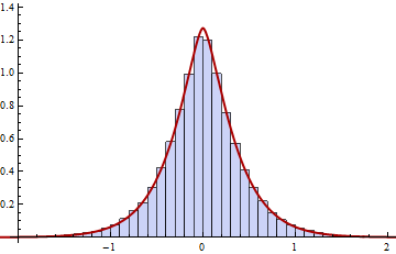
For instance, here is a plot of that PDF superimposed on the histogram of a random sample of $10^5$ such inner products where $\sigma=1/2$ and $n=3$:

It's harder to confirm the accuracy of the mgf from a simulation, but note (from the Binomial Theorem) that

$$(1 + t^2 \sigma^4)^{-3/2} = 1-\frac{3 \sigma ^4 t^2}{2}+\frac{15 \sigma ^8 t^4}{8}-\frac{35 \sigma ^{12} t^6}{16}+\frac{315 \sigma ^{16} t^8}{128}+\ldots,$$

from which we may read off the moments (divided by factorials). Due to the symmetry about $0$, only the even moments matter. For $\sigma=1/2$ we obtain the following values, to be compared to the raw moments of this simulation:

 k    mgf           simulation/k!
 2    0.09375       0.09424920
 4    0.00732422    0.00740436
 6    0.00053406    0.00054128
 8    0.00003755    0.00003674
10    2.58 e-6      2.17 e-6

As to be expected, the high moments of the simulation will begin departing from the moments given by the mgf; but at least up through the tenth moment, there is excellent agreement.

---

Incidentally, when $n=2$ the distribution is bi-exponential.

---

To handle the general case, begin by noting that the inner product is a coordinate-independent object. We may therefore take the principal directions (eigenvectors) of $\Sigma$ as coordinates. In these coordinates the inner product is the sum of independent products of independent Normal variates, each component distributed with a variance equal to its associated eigenvalue. Thus, letting the nonzero eigenvalues be $\sigma_1^2, \sigma_2^2, \ldots, \sigma_d^2$ (with $0 \le d \le n$), the mgf must equal

$$\left(\prod_{i=1}^d (1 - \omega^2\sigma_i^4)\right)^{-1/2}.$$

To confirm that I made no error in this reasoning, I worked out an example where $\Sigma$ is the matrix

$$\left( \begin{array}{ccc} 1 & \frac{1}{2} & -\frac{1}{8} \\ \frac{1}{2} & 1 & -\frac{1}{4} \\ -\frac{1}{8} & -\frac{1}{4} & \frac{1}{2} \end{array} \right)$$

and computed that its eigenvalues are

$$\left(\sigma_1^2, \sigma_2^2, \sigma_3^2\right) = \left(\frac{1}{16} \left(17+\sqrt{65}\right),\frac{1}{16} \left(17-\sqrt{65}\right),\frac{3}{8}\right)\approx \left(1.56639,0.558609,0.375\right).$$

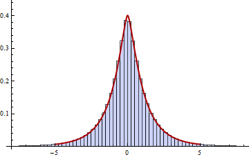
It was possible to compute the PDF by numerically evaluating the Fourier Transform of the characteristic function (as derived from the mgf formula given here): a plot of this PDF is shown in the following figure as a red line. At the same time, I generated $10^6$ iid variates $X_i$ from the Normal$(0,\Sigma)$ distribution and another $10^6$ iid variates $Y_i$ in the same way, and computed the $10^6$ dot products $X_i\cdot Y_i$. The plot shows the histogram of these dot products (omitting some of the most extreme values--the range was from $-12$ to $15$):

As before, the agreement is excellent. Furthermore, the moments match well through the eighth and reasonably well even at the tenth:

 k    mgf           simulation/k!
 2     1.45313       1.45208
 4     2.59009       2.59605
 6     5.20824       5.29333
 8    11.0994       11.3115
10    24.4166       22.9982

---

Addendum

(Added 9 August 2013.)

$f_{n,\sigma}$ is an instance of the variance-gamma distribution, which originally was defined as " the normal variance-mean mixture where the mixing density is the gamma distribution." It has a standard location ($0$), asymmetry parameter of $0$ (it is symmetric), scale parameter $\sigma^2$, and shape parameter $n/2$ (according to the Wikipedia parameterization).