In the case of $Z=XY\sim \text{Beta}(\alpha,1)$, the moment generating function (mgf) of $-\ln(XY)=-\ln X-\ln Y$ is
\begin{align}
M_{-\ln(XY)}(t)
&= E(e^{-t\ln Z})
\\ &=E(Z^{-t})
\\ &=\int_0^1 z^{-t}\alpha z^{\alpha-1}dz
\\ &= \frac{1}{1-t/\alpha}
\end{align}
which is the mgf of an exponentially distributed random variable with rate parameter $\alpha$.
Thus, if $X$ and $Y$ are iid, this means that $-\ln X$ and $-\ln Y$ must be Gamma distributed with shape parameter $1/2$ and rate parameter $\alpha$ (see wikipedia).
Backtransforming, the pdf of $X$ and $Y$ is
$$
f(x)=\sqrt{-\frac\alpha{\pi\ln x}}x^{\alpha-1}
$$
for $0\le x\le 1$.
A similar calculation in the general Beta$(\alpha,\beta)$-case leads to
$$
M_{-\ln(XY)}(t)=\frac{\Gamma(\alpha-t)\Gamma(\alpha+\beta)}{\Gamma(\alpha+\beta-t)\Gamma(\alpha)}
$$
and the mgf of $-\ln X$ and $-\ln Y$ would need to be the square root of this. But that is not the mgf of any known distribution and such a distribution (that when convolved with itself produces the target density) may not even exist.
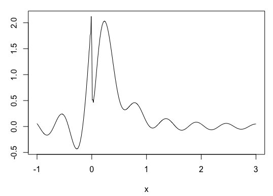
The pdf of $-\ln X$ can be computed via numerical integration of the inversion formula for the characteristic function $\varphi(t)=(M_{-\ln(XY}(it))^{1/2}$. This seems to produce valid pdfs for $\beta\le 2$ but for $\beta > 2$, the resulting function no longer appear to be a valid pdf:

R code:
library(pracma)
f <- function(x,phi,...) {
  integrand <- function(t) {
    exp(-1i*t*x)*phi(t,...)
  }
  line_integral(integrand,c(-300+0i,300+0i))/(2*pi)
}
f <- Vectorize(f,vectorize.args = "x")
phi <- function(t, alpha, beta) {
  sqrt(gammaz(alpha - 1i*t)*gammaz(alpha + beta)/(gammaz(alpha + beta - 1i*t)*gamma(alpha)))
}
x <- seq(-1,3,by=.01)
fx <- f(x, phi, alpha=3,beta=2.5)
plot(x,Re(fx),type="l")

